SOLUTIONS FOR CHAPTER 8
8.1 From (8.1),
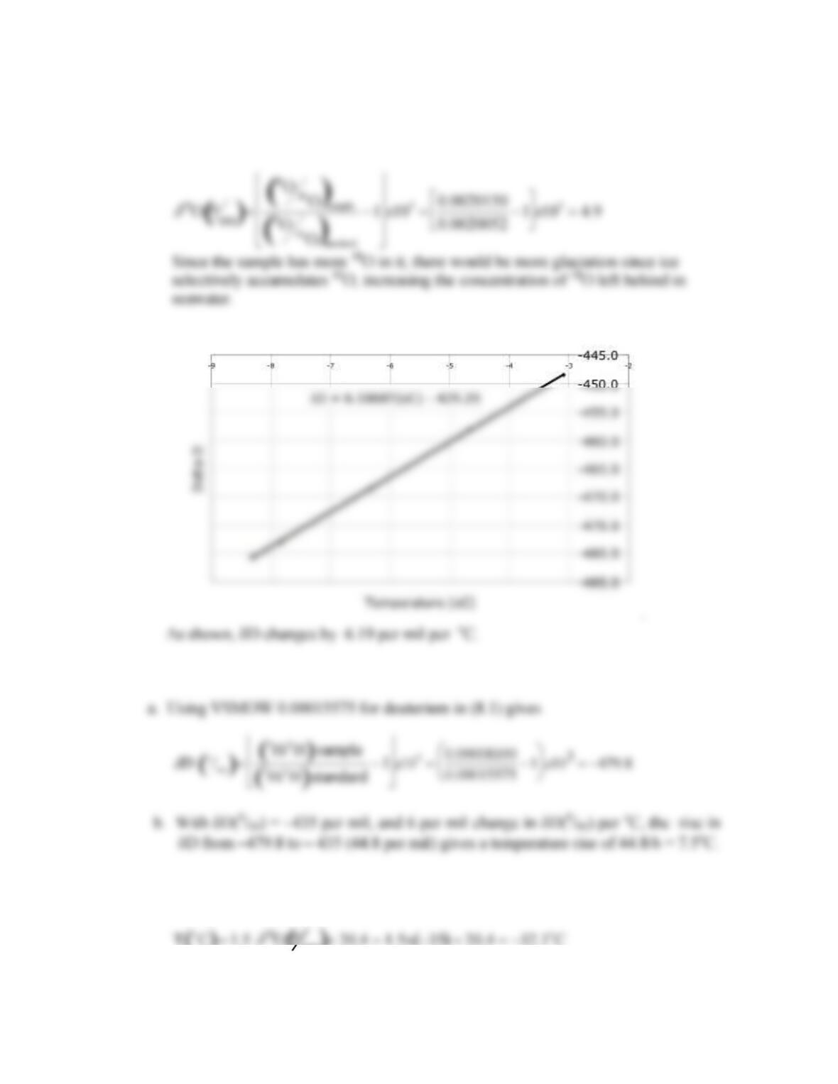
8.2 Plotting delta D versus temperature gives
8.3 An ice core with (2H/1H) = 8.100 x 10⁻⁵.
8.4 From the equation given for the ice core,
()
()
Pg. 8.1
(
)
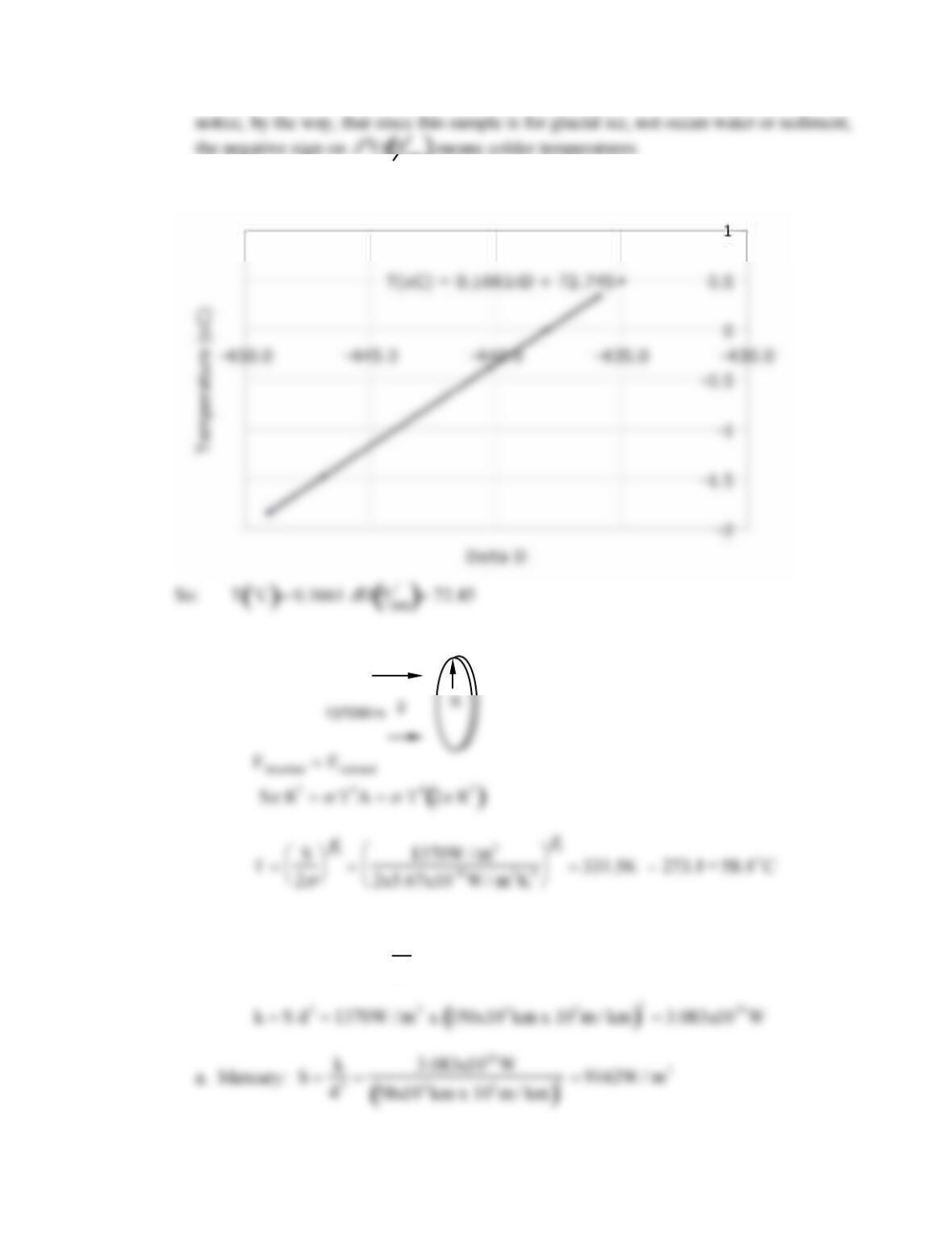
8.5 Plotting the ice core data for T(oC) and δD
8.6 The flat earth!
8.7 The basic relationship is S=k
d2. Using d and S for Earth from Table 8.2 lets us find k:
Pg. 8.2
b. The effective temperature (8.7) of Mercury would be:
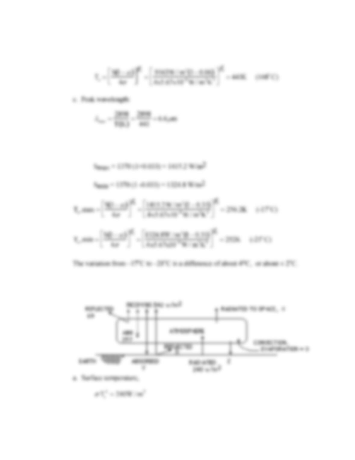
8.8 Solar flux variation of ±3.3%, gives a range of S
8.9 After a nuclear war:
Pg. 8.3

5.67x10⁻⁸W/m2K4
⎣
⎦
8.10 A 2-layer atmosphere:
342
107
X
Y
168
24 78
40
W
ZW
350
Z
T1
T2
390
Pg. 8.4

8.11 Hydrologic cycle:
8.12 Greenhouse enhanced earth:
100
342
67 24 78
30 Z
Y
X
291K
W
8.13 CO2 from 10 GtC/yr to 16 GtC/yr over 50 years, with initial 380 ppm and
A.F. = 40%. Since it is linear, the total emissions would be those at constant level
plus the area of a triangle rising by 6 Gt/yr:
Pg. 8.5
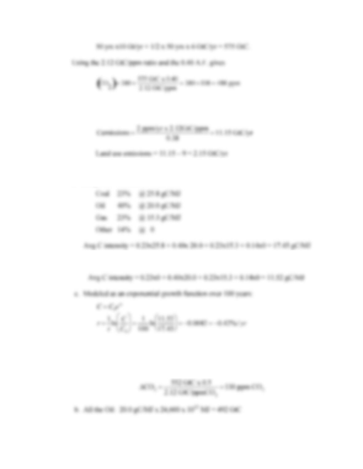
8.14 CO2 growing at 2 ppm/yr, fossil fuel and cement emissions at 9 GtC/yr, and A.F. of
38%. The remaining emissions due to land use changes are:
8.15 With 40% oil, 23% coal, 23% gas and 14% carbon free:
a. Using LHV values from Table 8.3:
b. Coal replaced by non-carbon emitting sources:
8.16 With resources from Table 8.4 and LHV carbon intensities from Table 8.3, A.F. = 50%:
a. All the N. Gas: 15.3 gC/MJ x 36,100 x 1012 MJ = 552,330 x 1012 gC = 552 GtC
Pg. 8.6
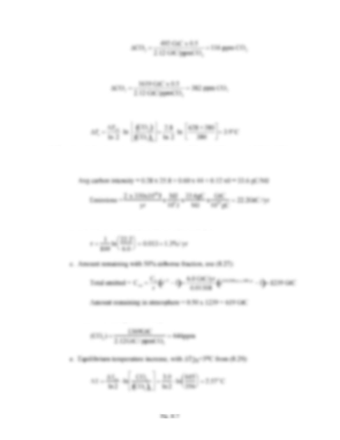
c. All the Coal: 25.8 gC/MJ x 125,500/2 x 1012 MJ = 1619 GtC
d. All three: 130 + 116 + 382 = 628 ppm CO2. From (8.29) with ΔT2X = 2.8oC:
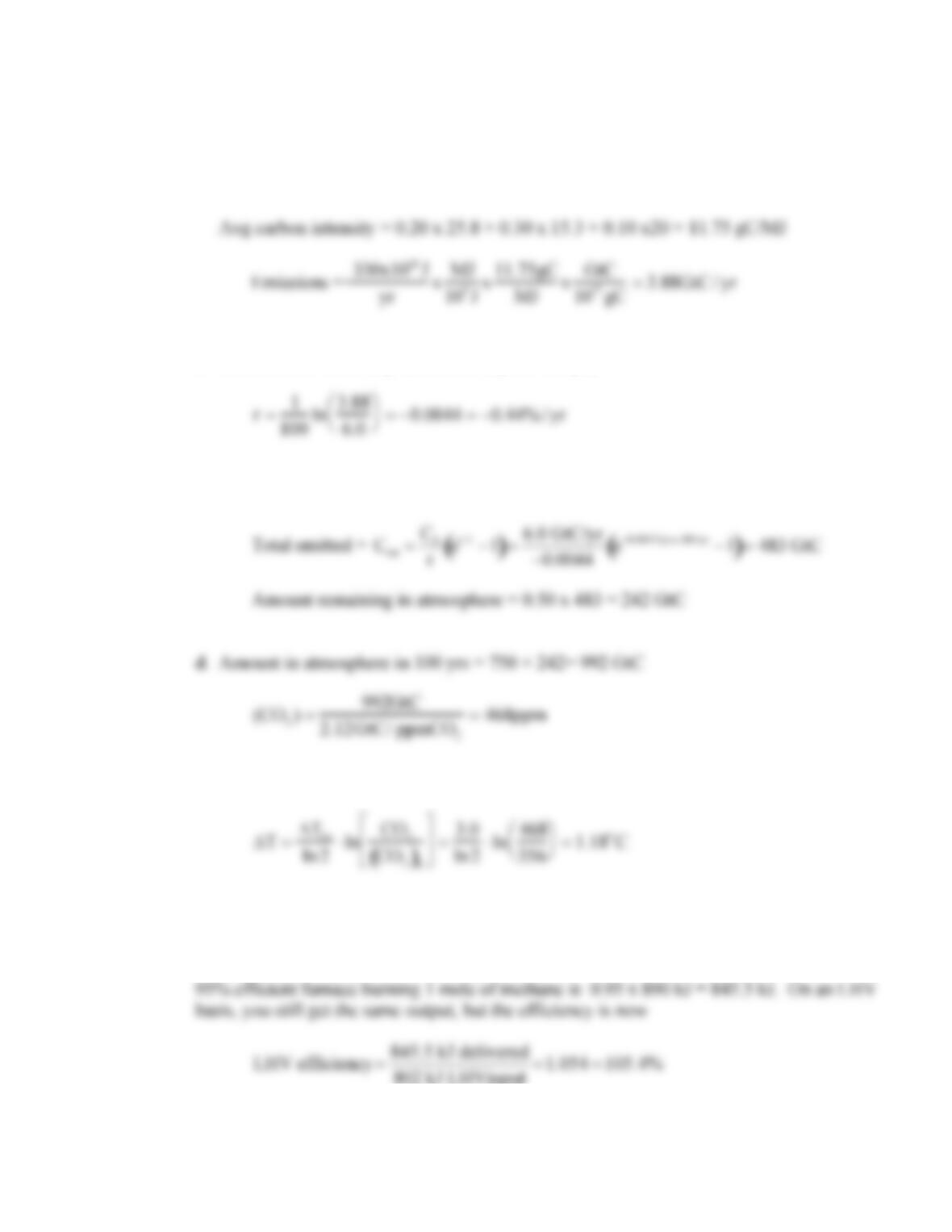
8.17 Out of oil and gas, demand = 2 x 330 EJ/yr, 28%coal, 60% syn gas/oil@44gC/MJ,
a. Carbon emission rate:
b. Growth from 6.0 GtC/yr to 22.2 GtC/yr in 100 yrs,
d. Amount in atmosphere in 100 yrs = 750 + 619 = 1369 GtC
8.18 Repeat of Prob. 8.17, but now conservation scenario:
a. Carbon emission rate:
b. Growth from 6.0 GtC/yr to 3.88 GtC/yr in 100 yrs,
c. Amount remaining with 50% airborne fraction, use (8.27):
e. Equilibrium temperature increase, with ΔT2x=3oC,
8.19. Finding LHV efficiency of a condensing furnace with 95% HHV efficiency.
From Example 8.4, HHV = 890 kJ/mol and LHV = 802 kJ/mol. The output of a HHV
Pg. 8.8
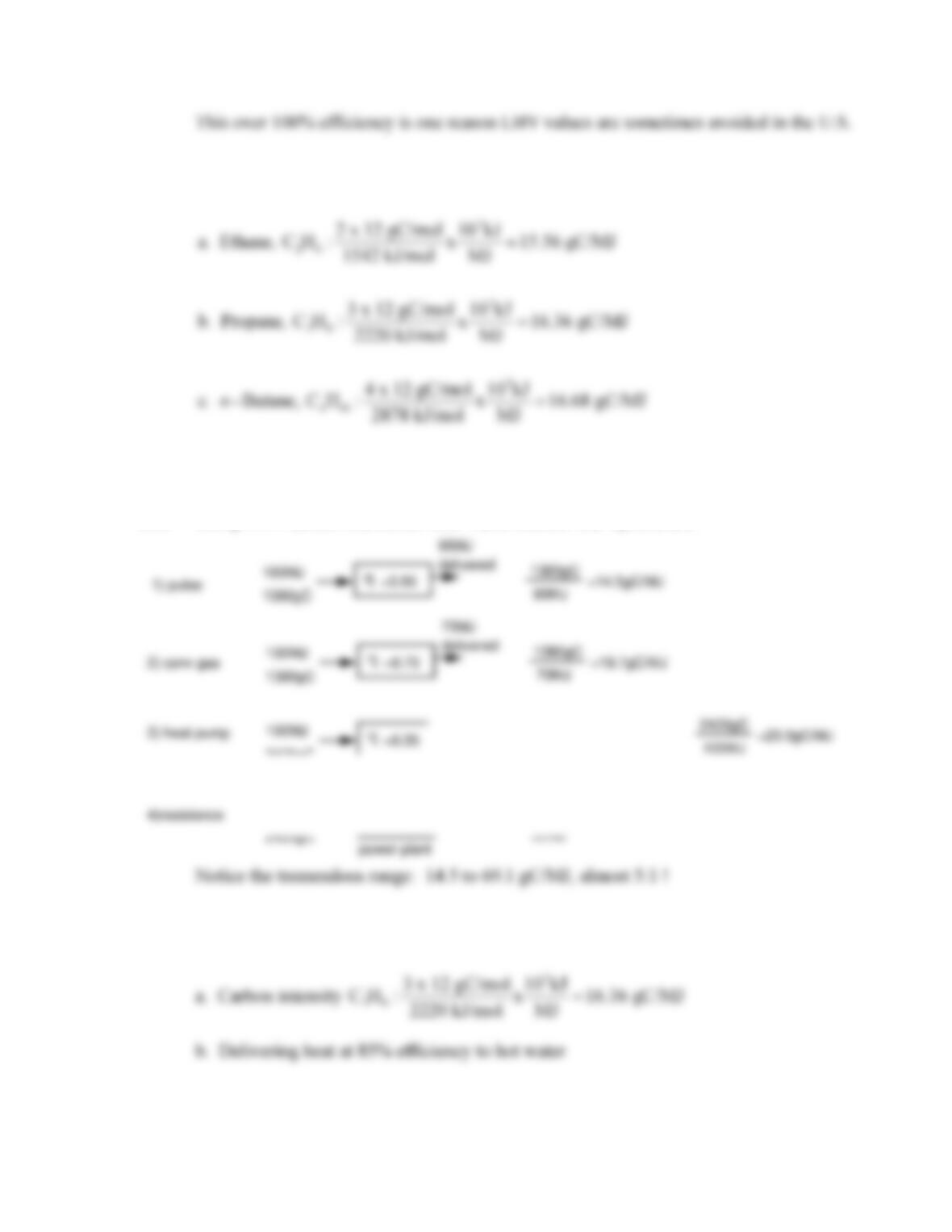
8.20 Finding HHV carbon intensities:
8.21 Using HHV carbon intensities from Table 8.3, the four options are:
8.22 Propane-fired water heater with 2200 kJ/mol vs Example 8.6:
Pg. 8.9
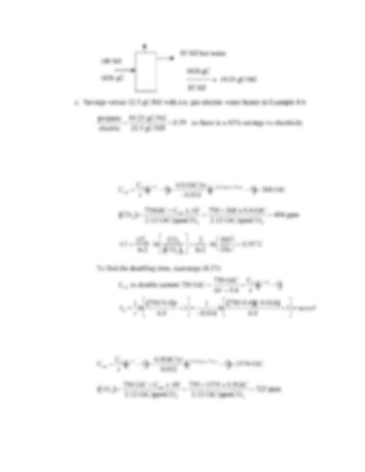
8.23 Initial CO2 = 356 ppm, 6 GtC/yr and 750 GtC; want 70 year scenario. Do it by scenario:
(A) Using r = 1.0 + 0.3 – 2.0 – 0.7 = -1.4%/yr in (8.27)
(B) r = 1.5 + 1.5 – 0.2 + 0.4 = 3.2%/yr
Pg. 8.10
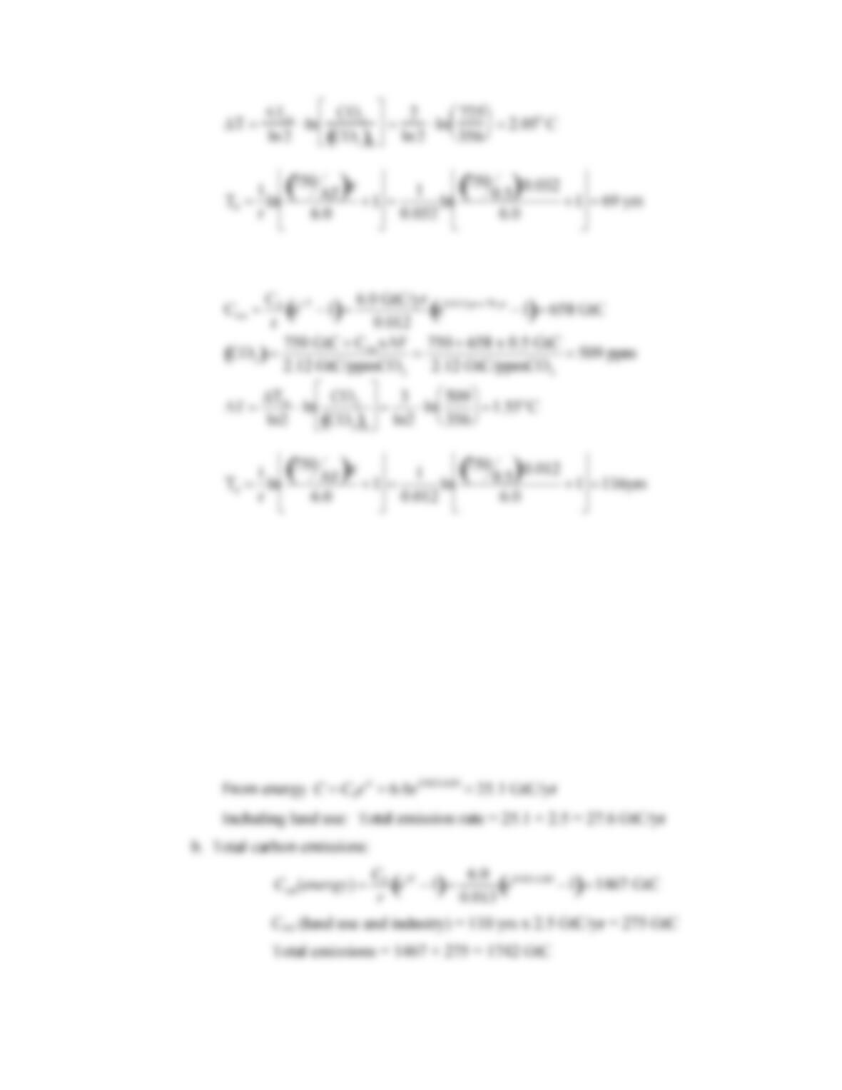
(C) r = 1.4 + 1.0 – 1.0 – 0.2 = 1.2%/yr
8.24 With 1990 6.0 GtC/yr + land use 2.5 GtC/yr and the following growth rates to 2100
Population growth rate dP/dt = 0.8%
Per capita GDP growth rate d(GDP/P)/dt = 1.3%
Final Energy per GDP growth rate =d(FE/GDP)/dt = – 0.7%
Primary Energy to Final Energy growth rate d(PE/FE)/dt = 0.1%
Carbon per unit of Primary Energy growth rate d(TC/PE)/dt = -0.2%
Carbon Sequestration growth rate d(C/TC)/dt = 0.0%
Total growth rate = 0.8 + 1.3 – 0.7 + 0.1 – 0.2 + 0.0 = 1.3%/yr
a. The carbon emission rate in 2100
Pg. 8.11