Pg. 7.14
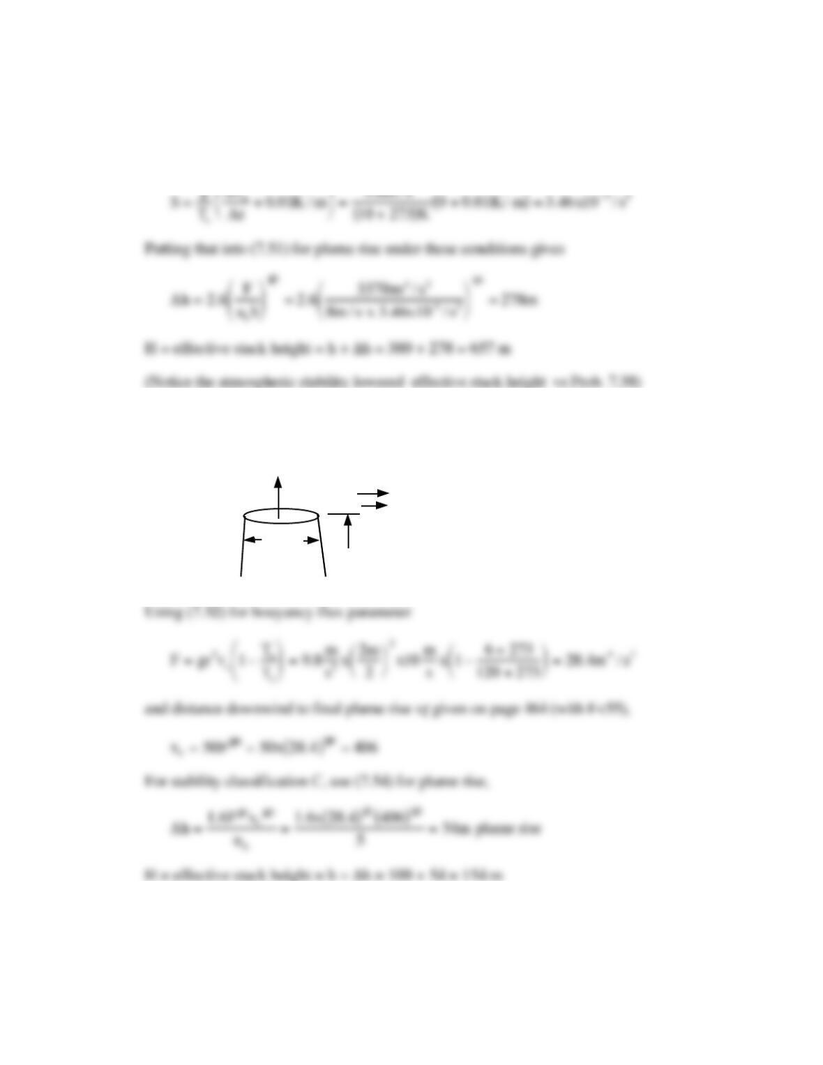
7.39 Repeat Problem 7.38 with a stable, isothermal atmosphere:
F = 3370 m4/s3 from Prob. 7.38. For isothermal atmosphere we can use (7.51) along a
stability parameter to estimate plume rise. The stability parameter (7.53) is
7.40 Cloudy summer day, stability classification C (Table 7.7),
120 C 10 m/s
2m
100m
6.0 C
o o
5 m/s
Pg. 7.15
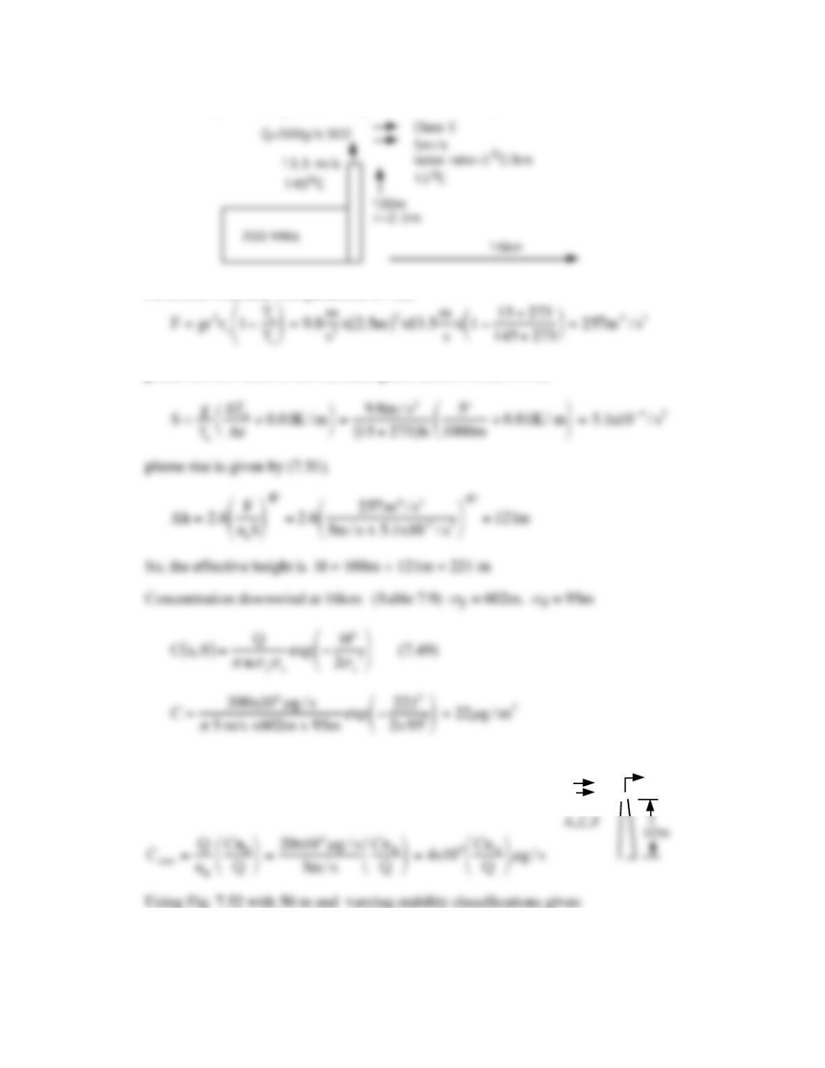
7.41 Power plant, find groundlevel pollution 16 km away. Need first find H.
First, find bouyancy flux parameter (7.52),
plume rise for stable (Class E) atmosphere needs S from (7.53),
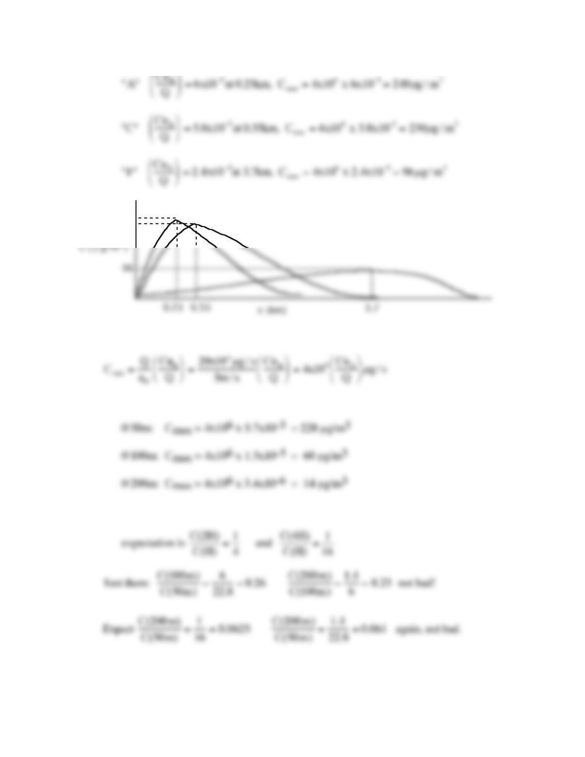
7.42 A 20 g/s source, 5 m/s, H = 50 m want peak concentrations Class A, C, F..
5 m/s
20 g/s
Pg. 7.16
3
240
230
7.43 H = 50m, 100m, 200m; Class C, 20 g/s, 5 m/s wind:
Using Fig. 7.52,
Do they drop as (1/H)2? That is,
Pg. 7.17
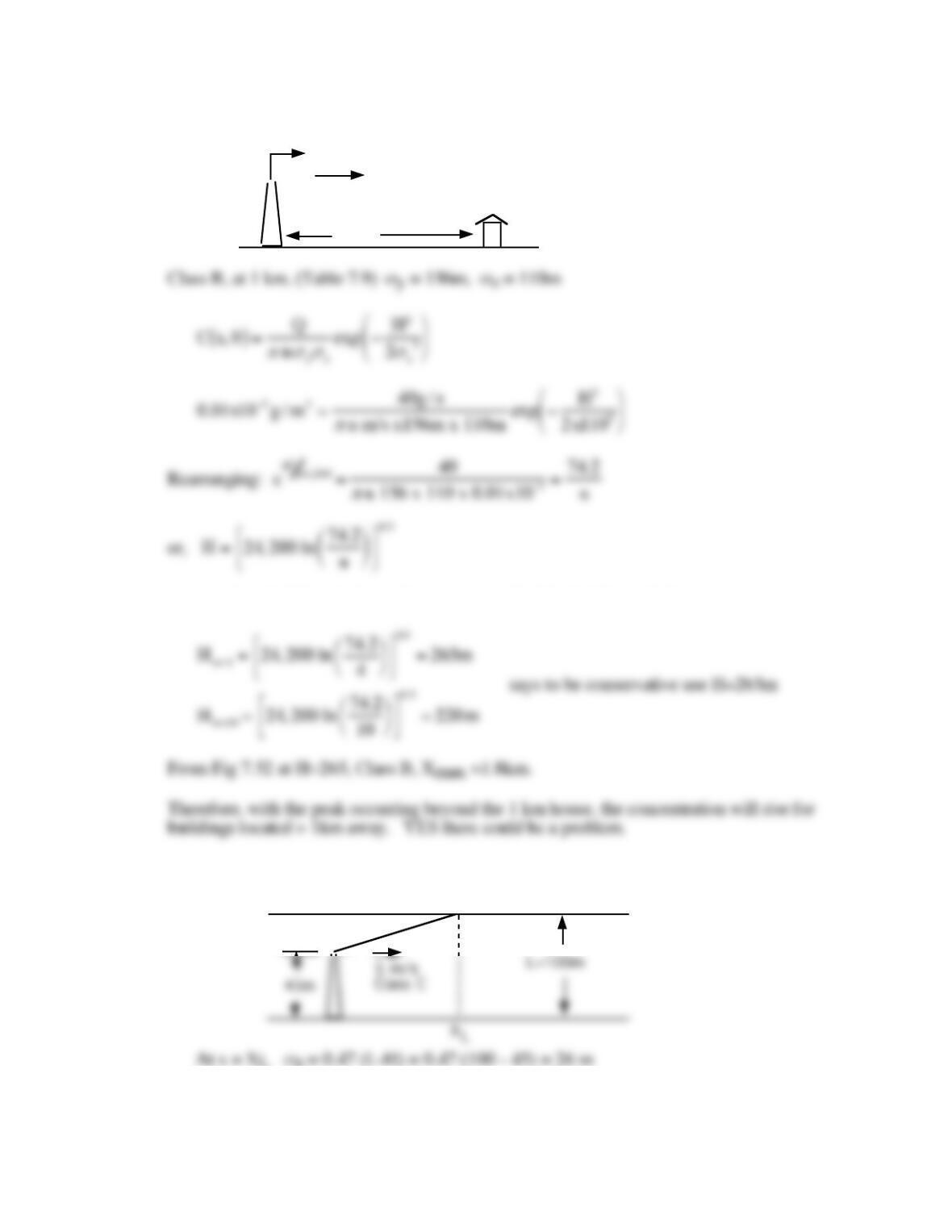
7.44 Paper mill emitting H2S, 1km away want 0.1 x odor threshold:
1 km
40 g/s
4-10m/s
Class B 0.01 mg/m3
so, at each end of the wind speed range we can find the height needed:
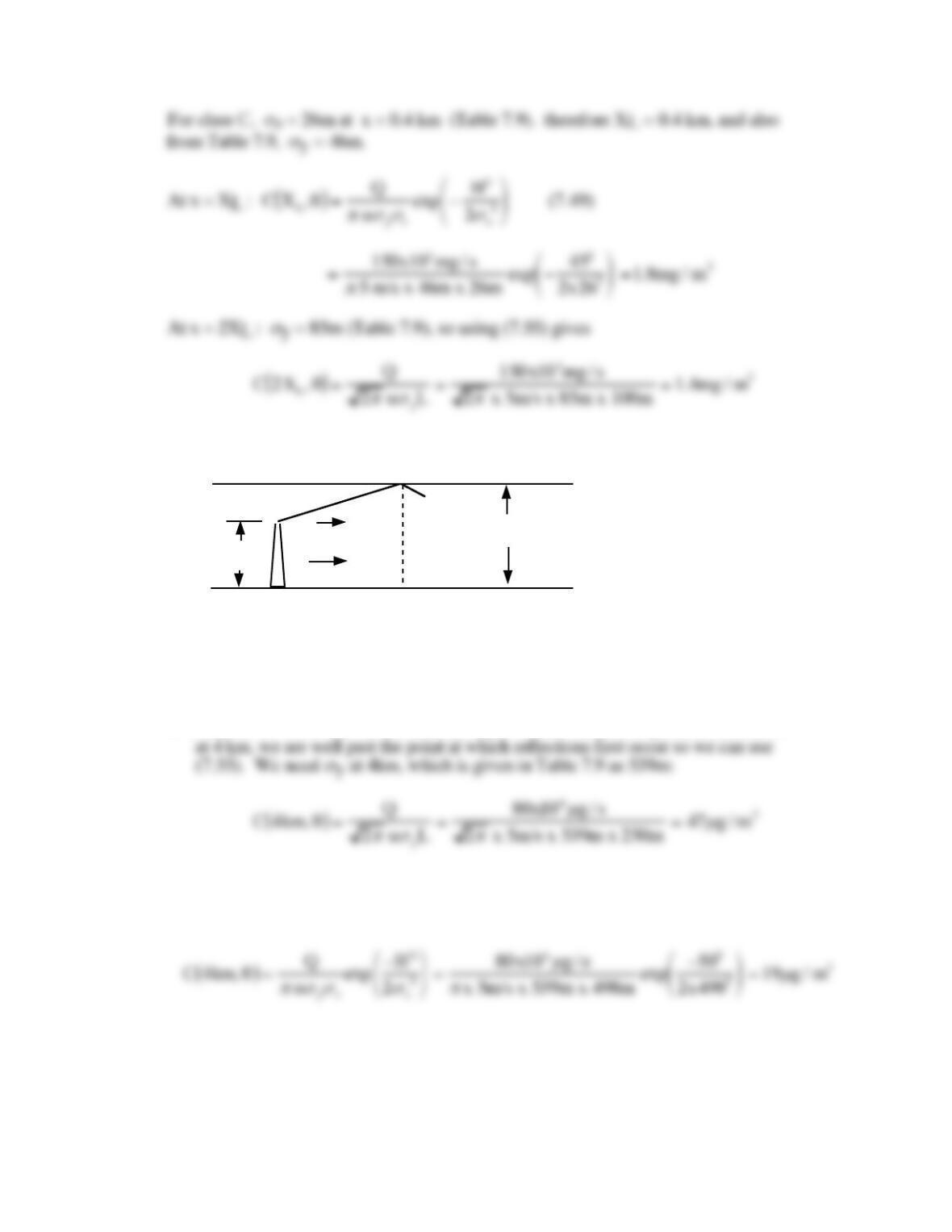
7.45 Stack under an inversion:
150 g/s
Pg. 7.18
7.46 Stack under an inversion layer:
50m
80 g/s 5 m/s
XL
L=250m
4 m/s
x=4km
C=?
We need the stability classification: Clear summer day, 4m/s, Table 7.7 says Class B.
at x = XL , (7.56) gives us σz = 0.47 (L-H) = 0.47 (250 – 50) = 94 m
a. From Table 7.9, at σz = 94m Class B, XL ≈ 0.9km. Since our point of interest is
b. Without the inversion layer, at 4km σz = 498m, σy = 539m so,
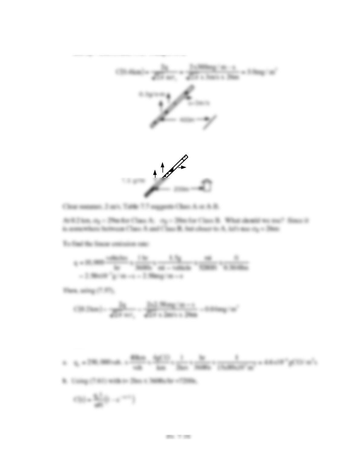
7.47 Agricultural burn. Clear fall afternoon, winds 3 m/s, so stability class “C” (Table 7.7),
and σz = 26m (Table 7.9). Using (7.57),
7.48 A freeway modelled as a line source:
10,000
vehicles/hr u=2m/s
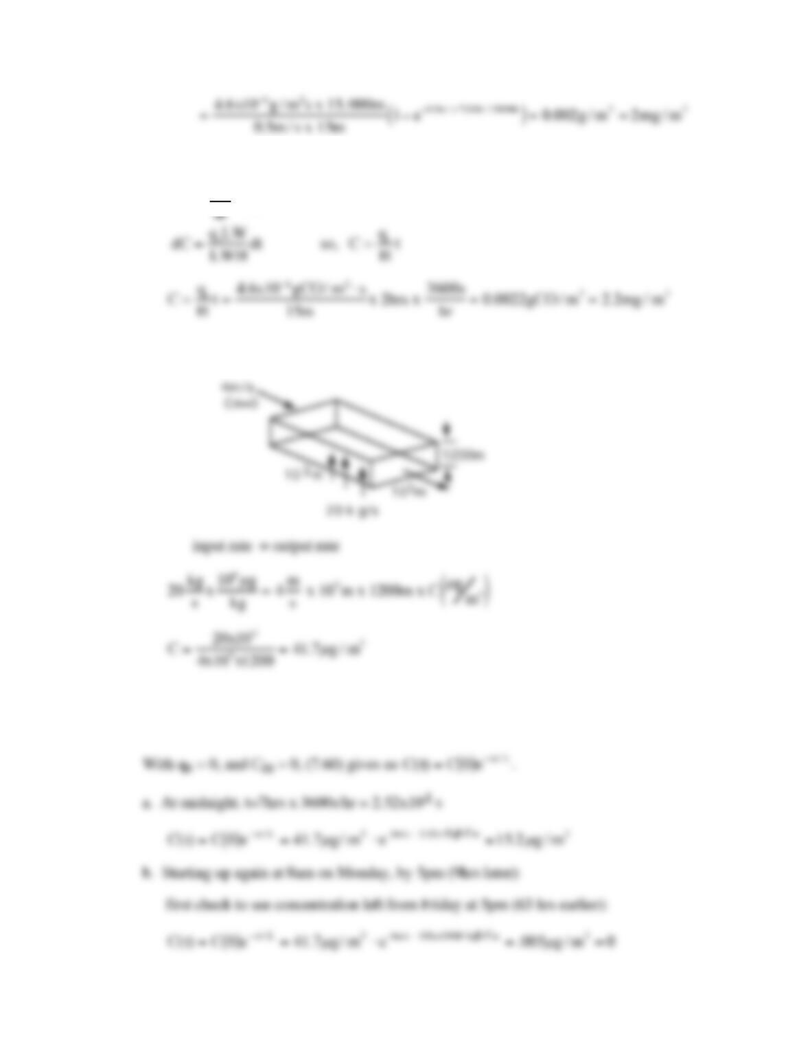
7.49 Box model, 250,000 vehicles between 4 and 6pm, driving 40km ea, emitting 4g/km
CO.
Pg. 7.20
c. With no wind, go back to (7.58) and solve the differential equation:
LWH dC
7.50 Box model, 105 m on a side, H=1200m, u=4m/s, SO2=20kg/s, steady state:
7.51 Assume steady-state conditions were achieved by 5pm Friday so that from Problem
7.50, C(0) = 41.7 µg/m3.
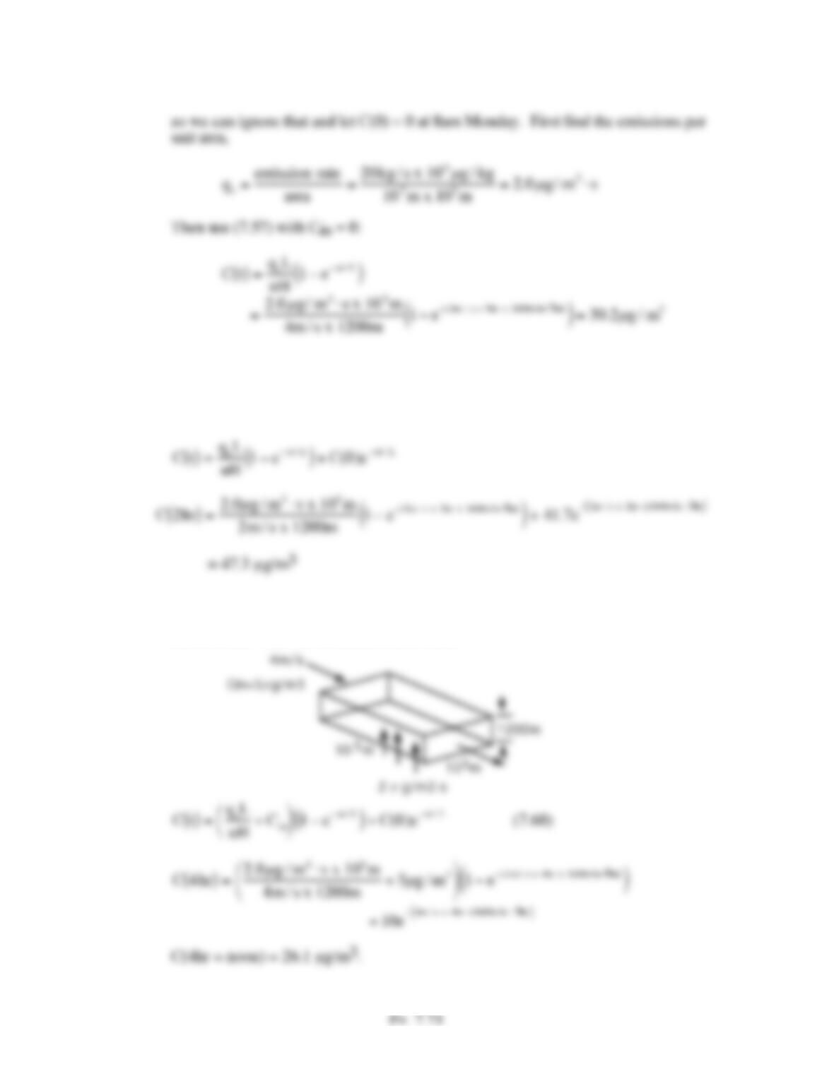
7.52 Steady-state conditions from Prob 7.50, wind drops to 2 m/s, 2hrs later:
From Prob. 7.50, emission rate qs = 2.0 µg/m2-s, and C = 41.7µg/m3. Using (7.60),
7.53 Modified Prob. 7.50, now incoming air has 5 µg/m3 and there are 10 µg/m3 already
there at 8am. Find the concentration at noon:
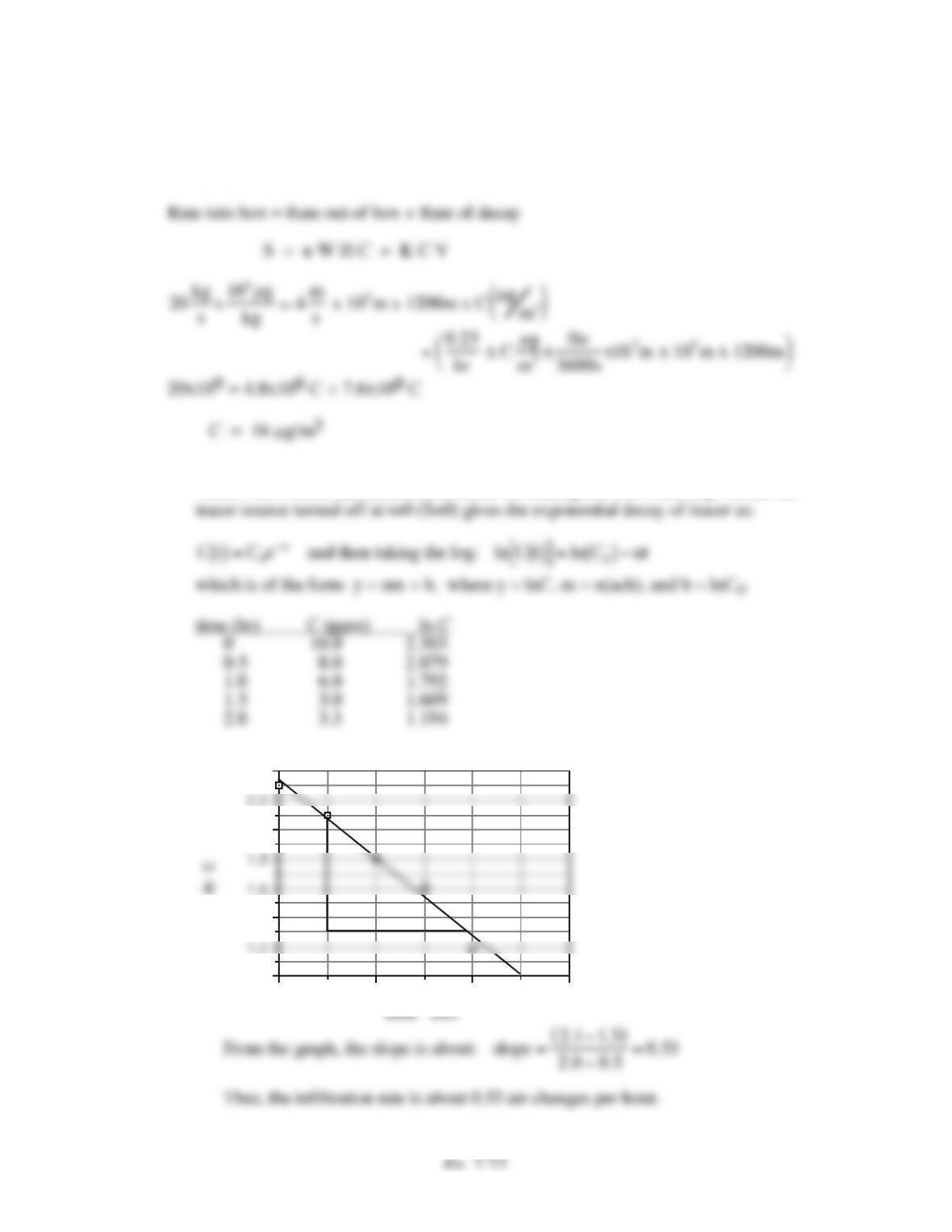
7.54 Now using conditions of Prob 7.50, but for a nonconservative pollutant with
K=0.23/hr:
7.55 Starting with (7.64) and using the special conditions of this tracer-gas study; that is, a
conservative tracer (K=0), no tracer in the air leaking into the room (Ca=0), and the
3210
1.0
1.4
2.0
2.4
Pg. 7.23
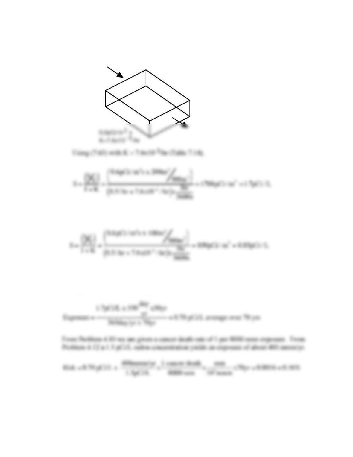
7.56 Infiltration 0.5ach, 500m3 volume, 200 m2 floor space, radon 0.6pCi/m2s:
0.5 ach
V=500m3
7.57 Same as Problem 7.56 but have half as much ground-floor area to let radon in, so:
7.58 From Problem 7.56, the radon concentration is 1.7 pCi/L. Using a residential
exposure factor of 350 days/yr from Table 4.10
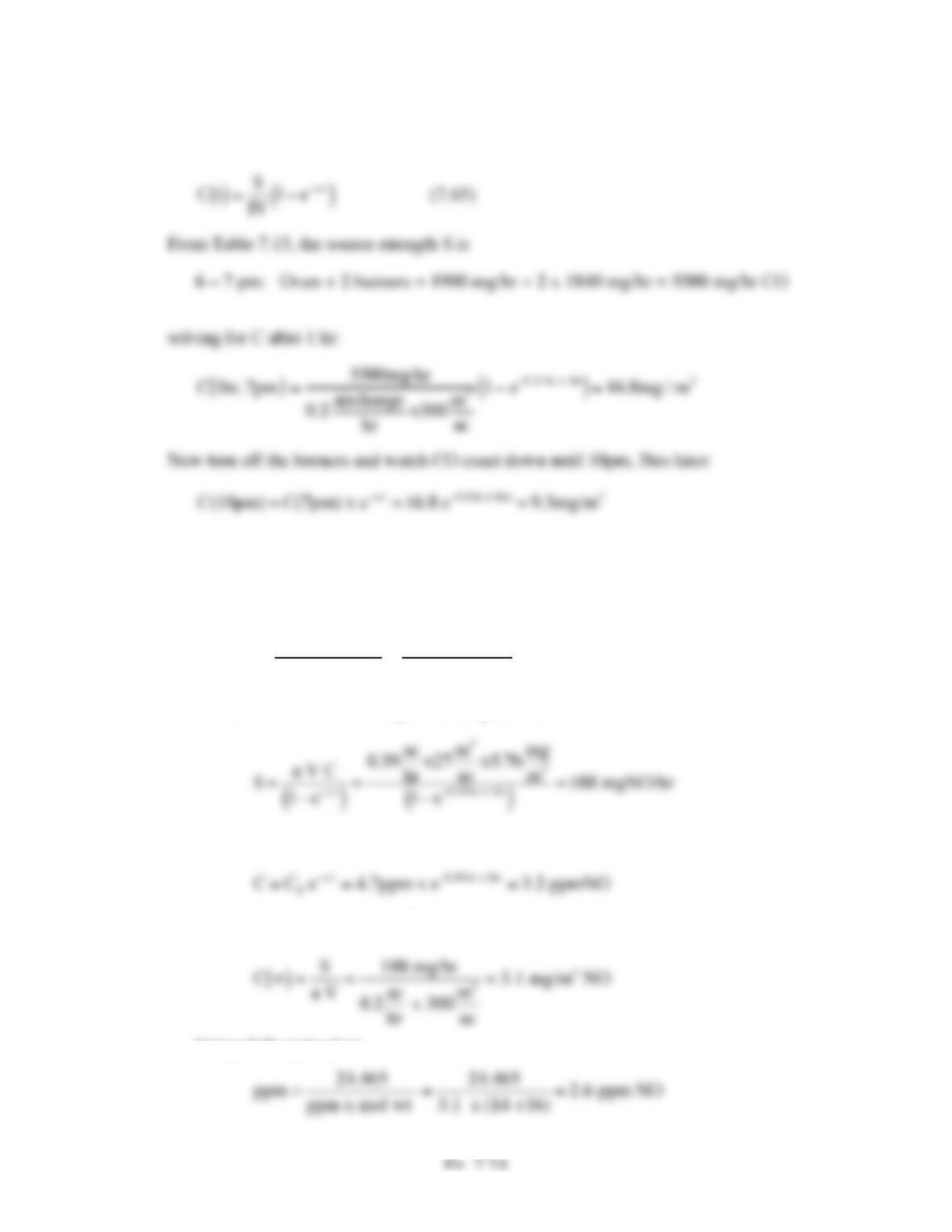
7.59 A 300m3 house, 0.2ach, oven+2burners 6pm to 7pm, find CO at 7pm and and 10pm.
For these circumstances, (7.65) is appropriate:
7.60 n = 0.39 ach, V = 27m3, after 1-hr NO = 4.7ppm. Find source strength, S:
First convert NO in ppm to mg/m3 using (1.9) and assuming T=25oC,
mg / m3=ppm x mol wt
24.465 =4.7 x 14 +16
( )
24.465 =5.76mg / m3
a. To find the NO source strength, rearrange (7.65)
b. 1-hr after turning off the heater,
c. In a house with 0.2 ach, 300m3,
Using (1.9) again gives
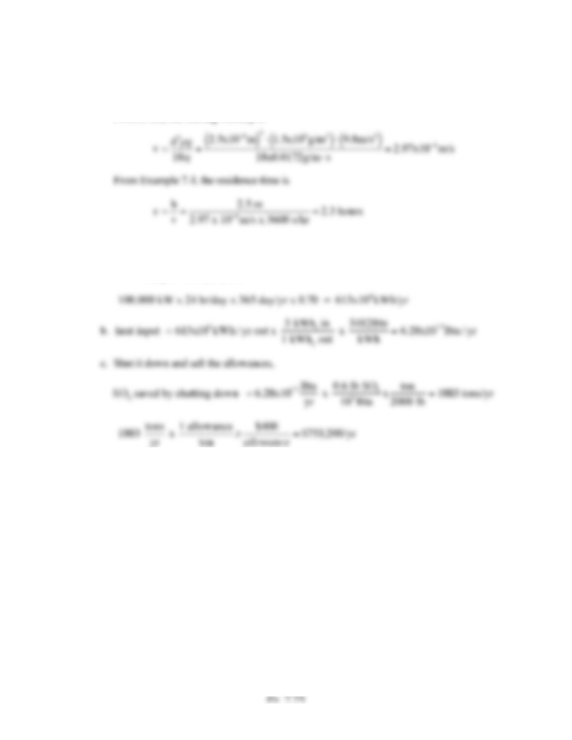
7.61 Find the settling velocity of 2.5-micron particles having density 1.5×10⁶ g/m3. In a
room with 2.5-meter-high ceilings, use a well-mixed box model to estimate the
residence time of these particles.
From (7.24) the settling velocity is
7.62 100,000 kW coal plant, 33.3% efficient, CF = 0.70,
a. Electricity generated per year,