QUESTIONS (10, PART A)
Flood Frequency in the Seattle/Tacoma area
Questions 1-11 investigate recurrence intervals, 100-year floods, and changing flood frequencies for
two watersheds in the state of Washington. These data are slightly modified from U.S. Geological
2. Use the formula and determine the recurrence interval of each of the 11 floods. Write the
results for each year in the “recurrence interval” column.
See the completed table.
Mercer Creek – Data Set 1 Mercer Creek – Data Set 2
Year Peak Flood
Discharge (in CFS)
Rank (1 is
greatest)
Recurr.
interval
Year Peak Flood
Discharge (in CFS)
Rank (1 is
greatest)
Recurr.
interval
1957 180 9 1.3 1979 518 5 2.4
1958 238 2 6.0 1980 414 7 1.7
Green River- Data Set 1 Green River – Data Set 2
Year Peak Flood
Discharge (in CFS)
Rank (1 is
greatest)
Recurr.
interval
Year Peak Flood
Discharge (in CFS)
Rank (1 is
greatest)
Recurr.
interval
1941 9310 10 1.2 1976 4490 11
1.1
1942 10900 7 1.7 1977 9920 4 3.0
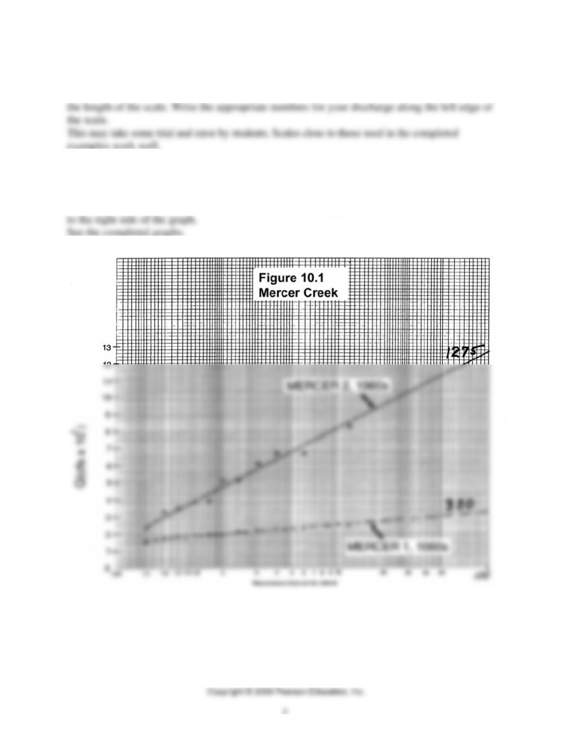
Questions 3-6 refer to Figure 10.1
3. Determine an appropriate vertical scale for your discharge data. The vertical scale should be
chosen such that the numbers you plot from the data above fill about one-half or slightly more of
4. Plot the discharge and recurrence interval for each of your 11 floods.
See the completed graphs.
5. Draw a best-fit straight line, not a dot-to-dot curve, through the data points. Extend your line
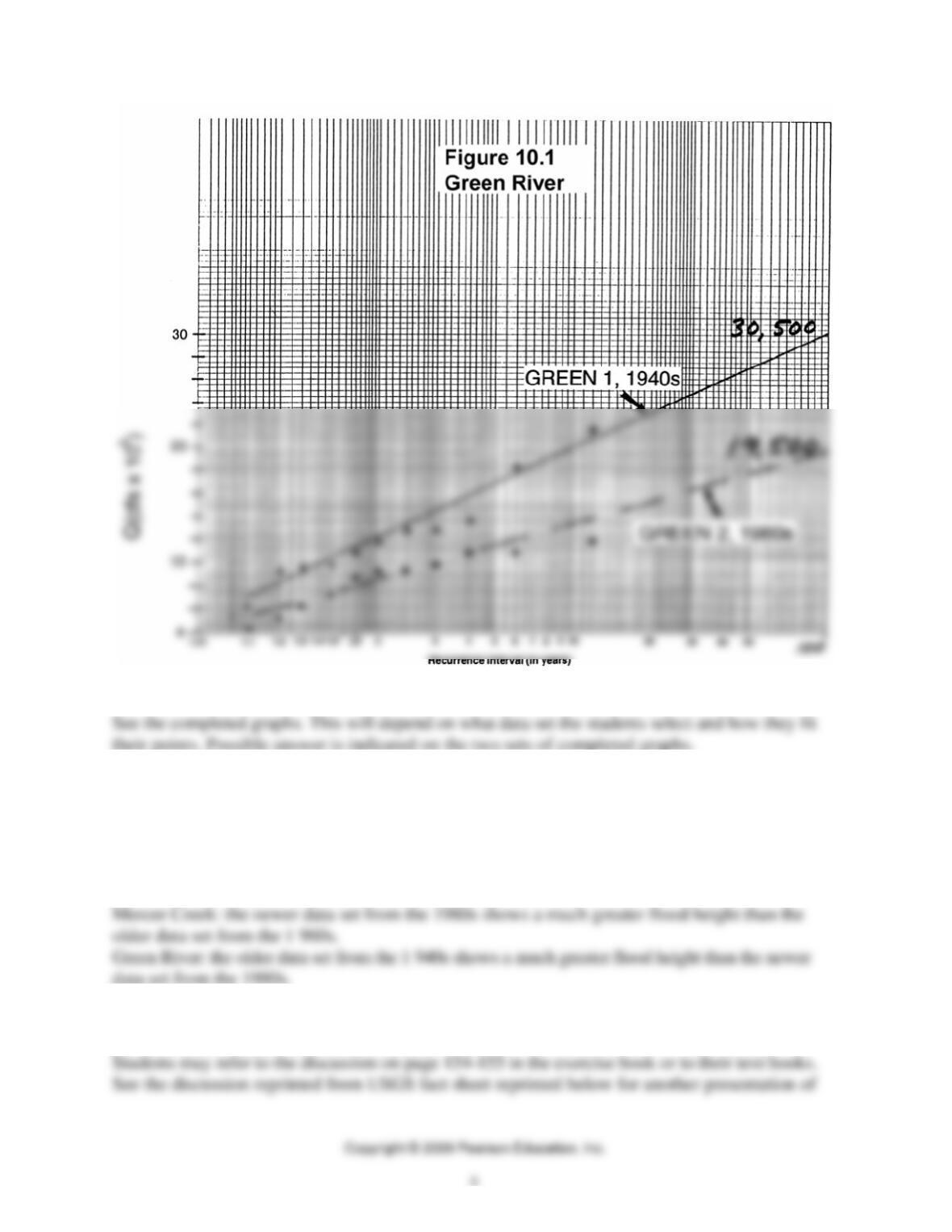
6. Based on your data, what is the predicted discharge for a 100-year flood?
7. Either find someone who has plotted the second set of data for your stream, or repeat
questions 1 through 6 to determine the predicted discharge for a 100-year flood, using the second
set of data for your stream. (You may plot the second set of data on Figure 10.1; note that
depending on your choice of numbers for the first plot, you may need to have a second set of
values on the vertical axis.) How does your prediction made in Question 6 compare with the
answer from the other set of data for the river you plotted?
8. Suggest possible human activities in the watershed that could have caused the differences in
predicted floods that result from the two sets of data.

9. When you have completed interpretation of the stream you selected, find students who have
done the other stream. How do their data compare with yours? What human activities did they
suggest for the changes in flood predictions they discovered?
Students here may be confused. Whichever trend they see in their data (is it newer or older
10. Based on the flood predictions for all four data sets, what does the contrast in predicted flood
discharges imply about the usefulness of the 100-year flood as a legal designation for these two
streams?
Students may reach their own conclusions, but geologically there does not seem to be much
11. What information do you need to know if you are about to buy a house that is located
adjacent to, but just outside of, the 100-year floodplain?
What is happening upstream? Development that increases flooding or dams that decrease
flooding? How much undeveloped land is there that could become impervious?
Large Floods in the United States
Data in Table 10.2, partly from the U.S. Army Corps of Engineers, show the damages suffered
Do Questions 12–16, which refer to Table 10.2.
12. On Figure 10.2, place a point for each decade to show monetary flood loss (in billions of
dollars) for each decade. What is the general trend in flood loss in the United States between
1900 and 2000 as determined from Table 10.2 and your graph?
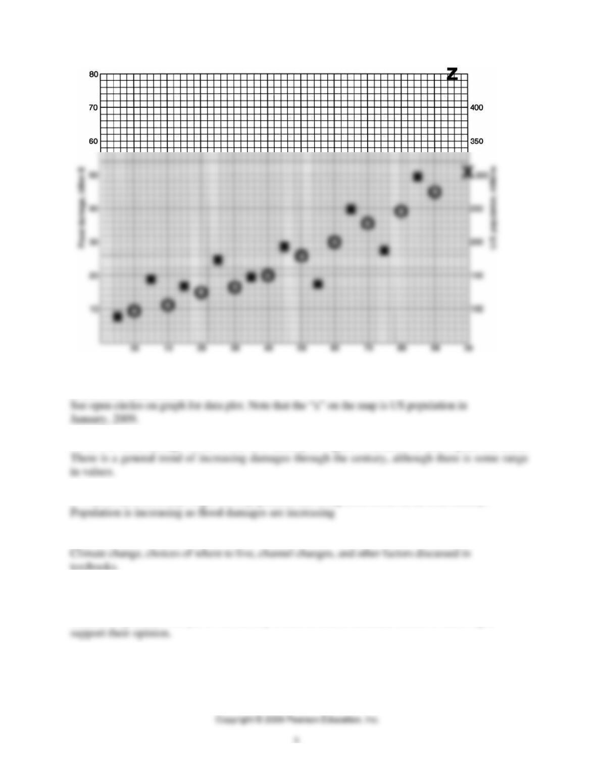
13. Now place an open circle for each decade to show the U.S. population in millions of people
at the end of each decade.
14. a. For flood damage losses in the 20th century in Figure 10.2, describe and explain the trend.
b. What is the role, if any, of growth in population and rising flood losses in the 20th century?
c. What other factors contribute to increased losses?
15. Discuss the effectiveness of flood mitigation in the 20th century with your lab group. Are
flood control systems effective?
Students may answer this yes or no, but they should be able to articulate scientific reasoning to
16. According to the Corps of Engineers (2000), for the decade of the 1 990s, the average damage
loss per year was about $5 billion. For the same period the average value of flood damage
reduction by projects per year is estimated at $20 billion. Using this information and that in the
graphs you plotted discuss the statement “Flood-control dams and levees have been effective in
reducing flood damage” and suggest additional measures for reducing flood damage.
An assumption in this statement is that flood-control dams have generally been used throughout
The Discharge/Area Ratio
Questions 17 and 18 investigate ranges in flood discharge (Q) with drainage basin size (A) for
several different sizes of rivers. This flood intensity comparison is based on data in Table 10.3,
which will be plotted in Figure 10.3.
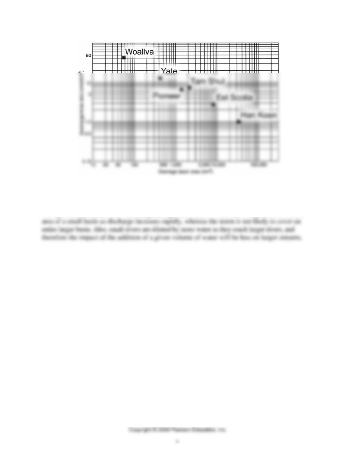
17. Use the flood records in Table 10.3 to calculate the discharge/area ratio for each river.
Record your calculation in the column on the table. Plot the calculated ratio against drainage-
basin area in Figure 10.3. Identify the six rivers that you are able to plot.
See table and graph below.
River
Name Location
Drainage Basin
Area (km2)
Maximum
Discharge, Q
(m3/s)
Q/A Ratio
(m3/s)/km2)
Woallva Hawaii 58 2,470 42.6
18. From your calculations and plots determine the general relationship between Q/A ratio and
drainage basin area. With increasing area of drainage basin, is there an increase or decrease in
the Q/A ratio? Briefly explain the reason for this.
The Q/A ratio decreases with increasing drainage basin area. A small storm may cover the entire
QUESTIONS 10, PART B
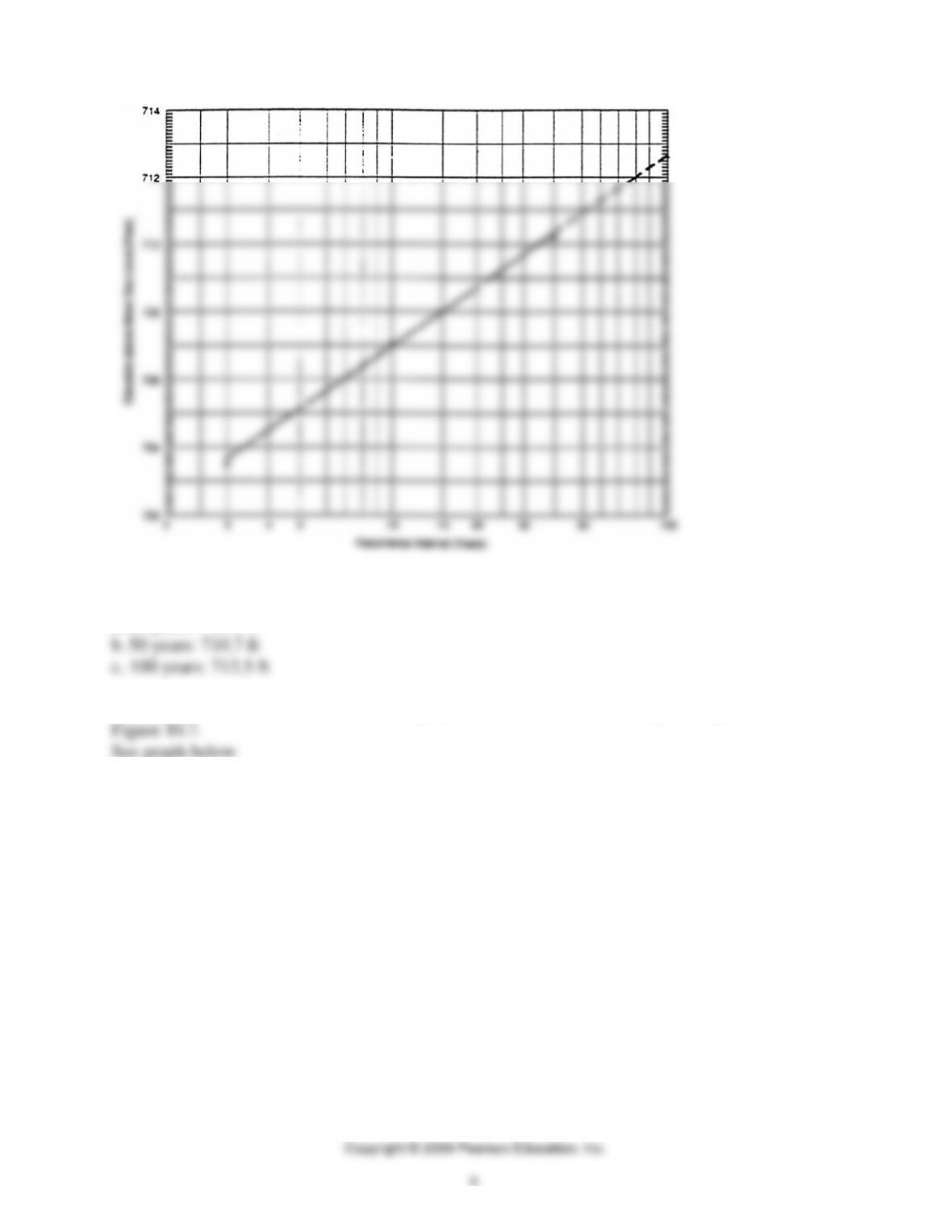
1. Using the data in Table 10.4 and the graph paper (Figure 10.6) plot the data and draw a
straight line for frequency of floods at Dillon Falls, Ohio. Use a dashed line beyond the 40-year
recurrence interval.
See graph below.
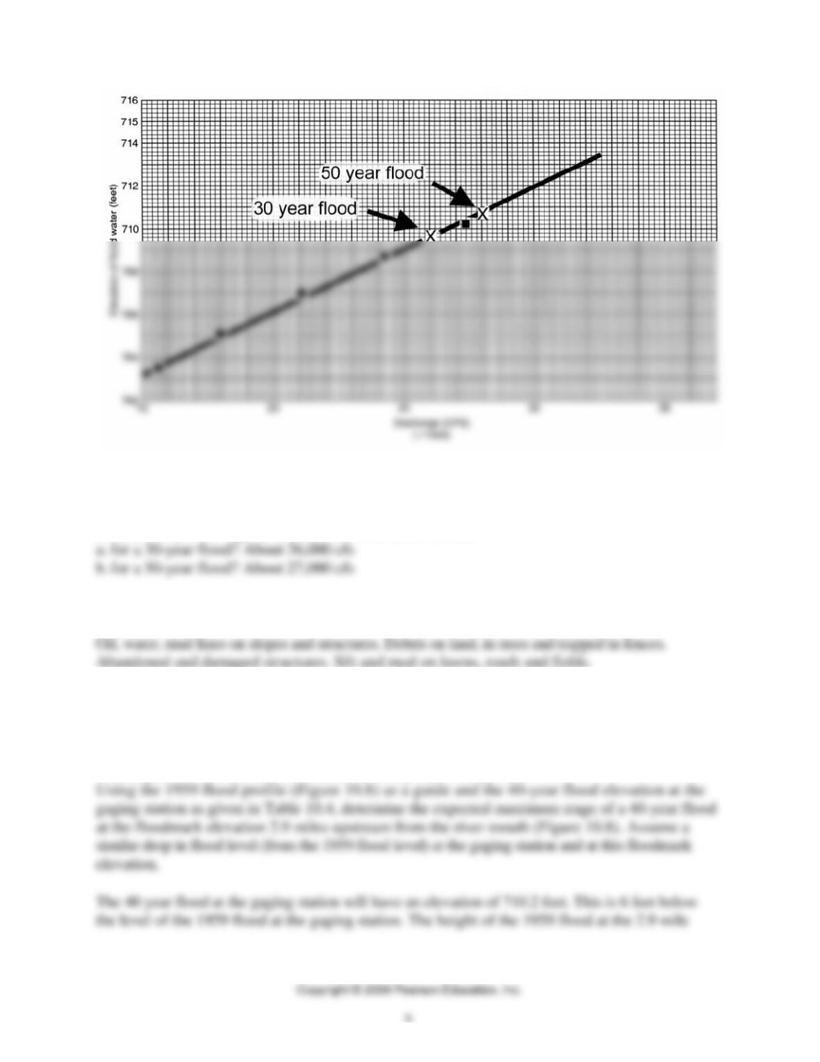
2. What are the expected elevations of the following floods at the Dillon gaging station as
determined from Figure 10.6?
a. 30 years: 709.6 ft
3. Using the data in Table 10.4 construct a graph of elevation versus discharge (rating curve) in
4. Discharge can be obtained for a flood of a given frequency by using information on the flood
frequency–elevation curve (Figure 10.6) and the rating curve (Figure 10.7). What is the expected
discharge at Dillon, Ohio
Students may have slightly different takes on a best fit line.
5. If you visit a flood area after the water recedes, what indications might there be on buildings,
trees, and land surfaces of the level of the flood maximum?
6. Figure 10.8 is a flood profile of the Licking River for the 1959 flood at Zanesville. Elevations
are plotted against the distance upstream from the mouth (in miles along the centerline of the
river). The maximum elevation of the 1959 flood at the gage given in the introduction. Profiles
of higher or lower floods can be plotted on this diagram, although backwater effects from the
Muskingum River and channel constrictions may affect the profile.

7. List several approaches that have been applied to reduce losses from river floods. (Consult
your notes, textbooks, or references, if necessary.) Group the approaches as either control of the
river and/or control of land use or human activity.
Control of the river might include dams, levees, channelization, dredging, and other physical
QUESTIONS (10, PART C)
1. Examine Table 10.5. Plot the cumulative rainfall for the sites in this table on Figure 10.9 and
draw in the lines of equal precipitation (isohyets) for 6, 8, and 10 inches.
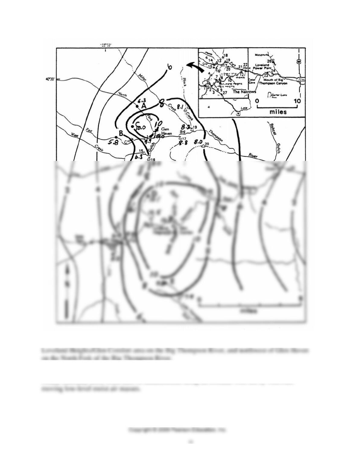
2. Where were the centers of precipitation?
3. What is the explanation for the intense, localized nature of this precipitation event?
Nearly stationary north-south lines of thunderstorms along the foothills were fed by westward