
Exercise 6
QUESTIONS PART A1
Epicenter
1. In Figure 6.2, use the time scale to determine the lag in arrival time between the P and S
waves at four stations: St. Louis, Missouri (SLM); Bloomington, Indiana (BLO); Minneapolis,
Minnesota (MNM); and Bowling Green, Ohio (BGO). The first major impulse on the left in the
2. To determine the distance from the earthquake to each seismograph station we must first
determine the time lag between P and S wave arrivals at a given distance from an earthquake, say
100 km, knowing the average velocities of the P and S waves. If the average velocity of the P
wave is 6.1 km/sec and the average velocity of the S wave is 4.1 km/sec, what is the time
required for each wave to travel 100 km? (It may help to think of this problem like a very fast
driving trip: if you want to go 100 km, and you drive at a rate of 6.1 km/sec, how long, in
seconds, will it take you to get to your destination?)
3. Using the data from Figure 6.2 and the equation in the exercise book, determine the distance to
the earthquake epicenter from each station and enter below.
SLM: 250–263 km
4. a. The epicenter of the earthquake can be pinpointed by drawing compass arcs from three of
the stations with radii corresponding to the distances calculated in Question 3. The intersection
of these radii marks the epicenter. Do this in Figure 6.3.
d. At what time did the earthquake occur? (Refer to Figure 6.2.)
Use the given velocities and determined epicenter-to-station distances to calculate the amount of
QUESTIONS 6, PART A2
1. Following are some historical descriptions of earthquakes (a–d). Such statements, made to
scientists or reporters, or recorded in diaries or on survey forms distributed by government
agencies, allow scientists to determine the intensity of an earthquake. Using the Modified
Mercalli Intensity Scale (Table 6.1), assign each of the quakes an intensity number. Pick the
lowest number exhibiting the characteristics given. The first quotation describes the observations

Intensity: VIII
b. “The shock seemed to be a sort of gentle swaying back and forth, causing hanging fixtures to
swing, but doing no damage.” (Iacopi, 1971)
Intensity: II-IV
2. Not all earthquakes occur in areas where high levels of risk have been identified. On July 27,
1980, an earthquake of Richter magnitude 5.1 shook Kentucky, Ohio, and adjacent states. The
earthquake epicenter was determined to be at latitude 38.2° N, longitude 83.9° W, near
Sharpsburg, Kentucky (approximately 30 miles southwest of the Ohio River town of Maysville,
Kentucky). It had a focal depth of 13 km. Damage to structures along the Ohio River in
Maysville, Kentucky, and in the Ohio communities of Aberdeen, Manchester, Ripley, and West
Union, consisted of chimneys being knocked down, cracks in plaster and concrete blocks, and
QUESTIONS 6, PART A3
1. The intensity of an earthquake is a measure of the impact of seismic shaking on the ground,
structures, and people. It is described on a scale of I to XII (in Roman numerals), where I is only
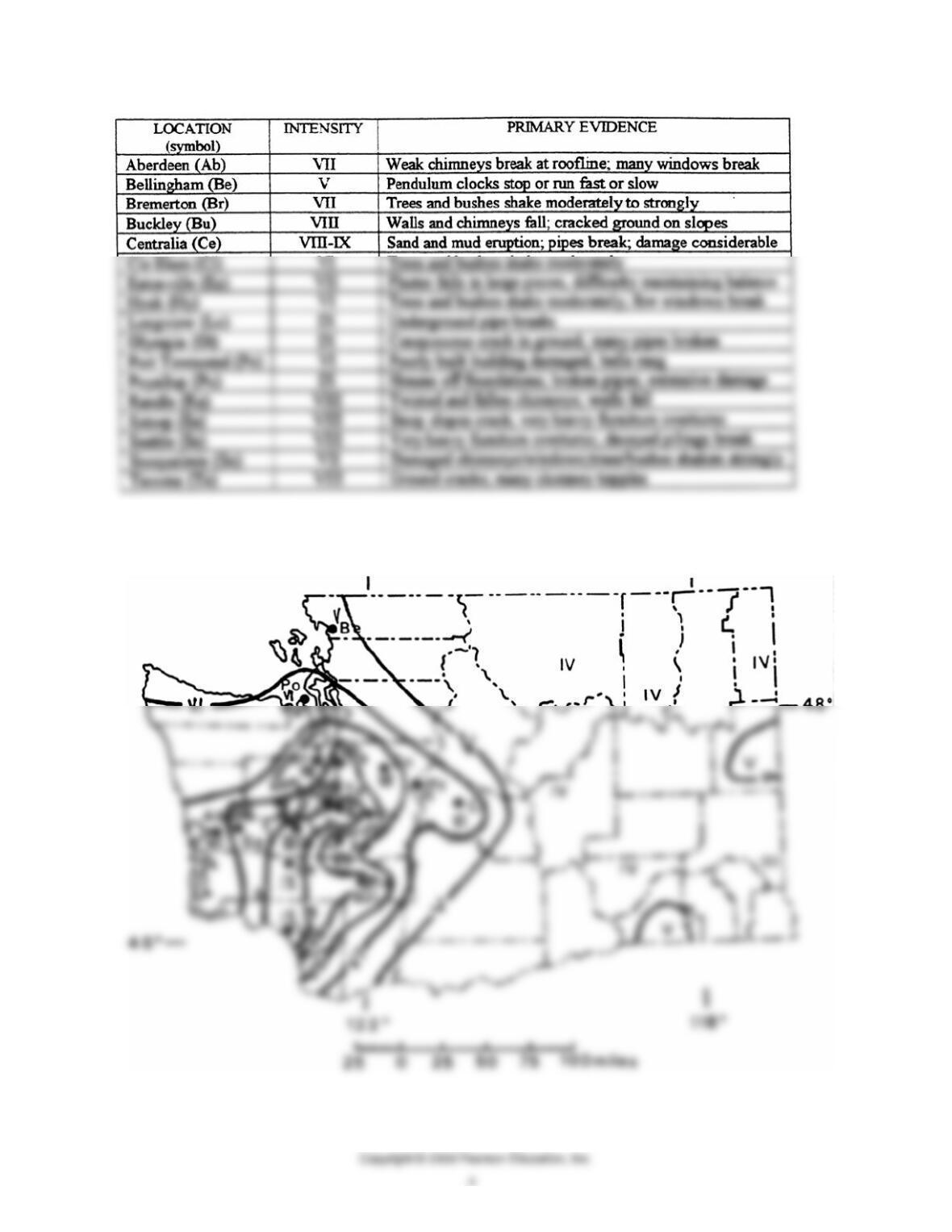
2. Place the intensity values from Table 6.3 on the map of Washington (Figure 6.4). Then draw
boundaries between these intensities to produce an isoseismal map.
See map below.
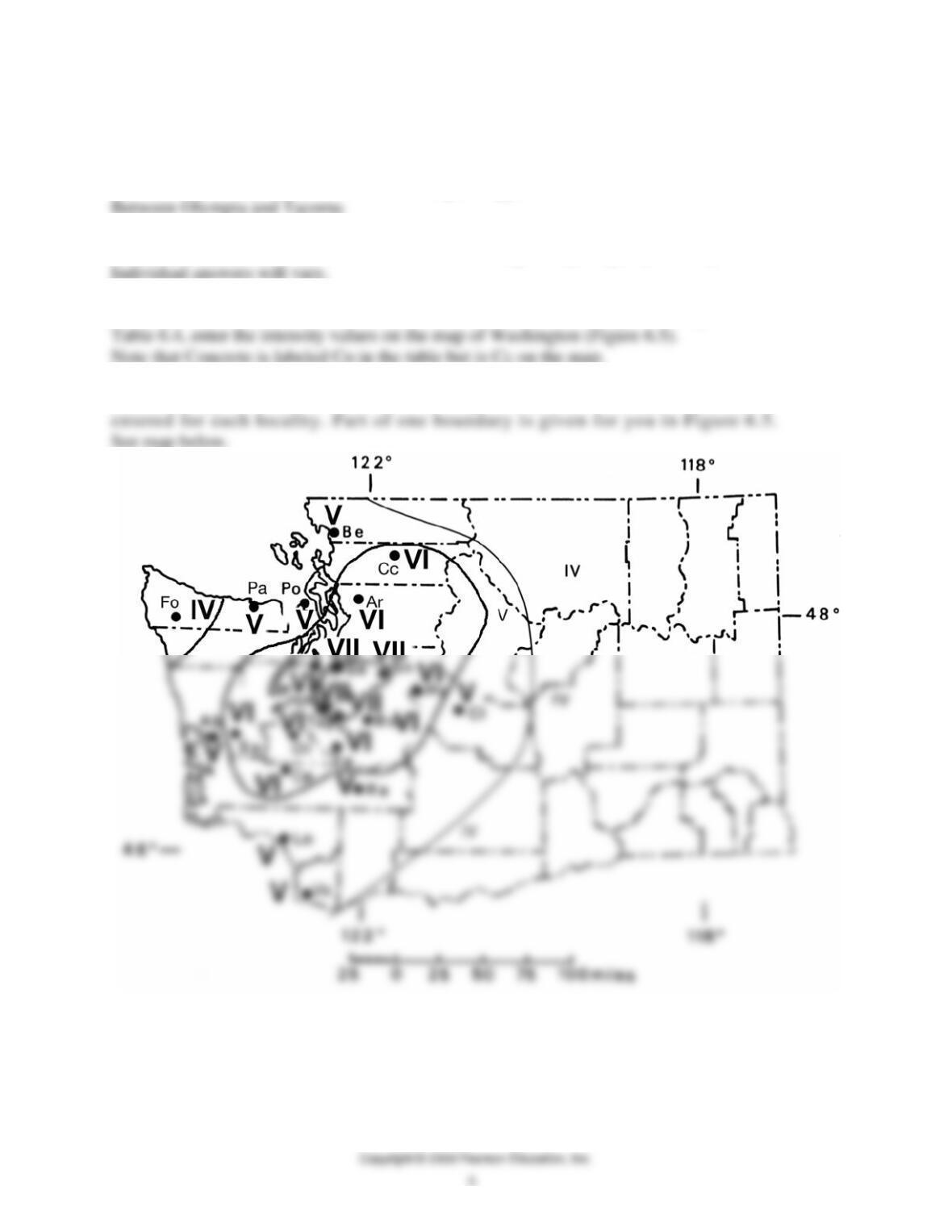
3. What was the maximum intensity from the 1949 earthquake?
IX
4. Where does the epicenter for the 1949 earthquake appear to have been?
5. What observation in Table 6.2 was the most interesting or surprising to you? Why?
6. Using intensity numbers from the April 29, 1965 western Washington earthquake shown in
7. Draw the approximate boundaries of the intensity zones as determined by the values you
8. a. What was the maximum intensity for the 1965 earthquake?
VII

9. On the Web you will find additional information on these two earthquakes (and others) at
1949 Earthquake 1965 Earthquake
Date April 13 April 29
b. You might still be curious about earthquake intensities. Below write a question for your TA or
QUESTIONS 6, PART A4
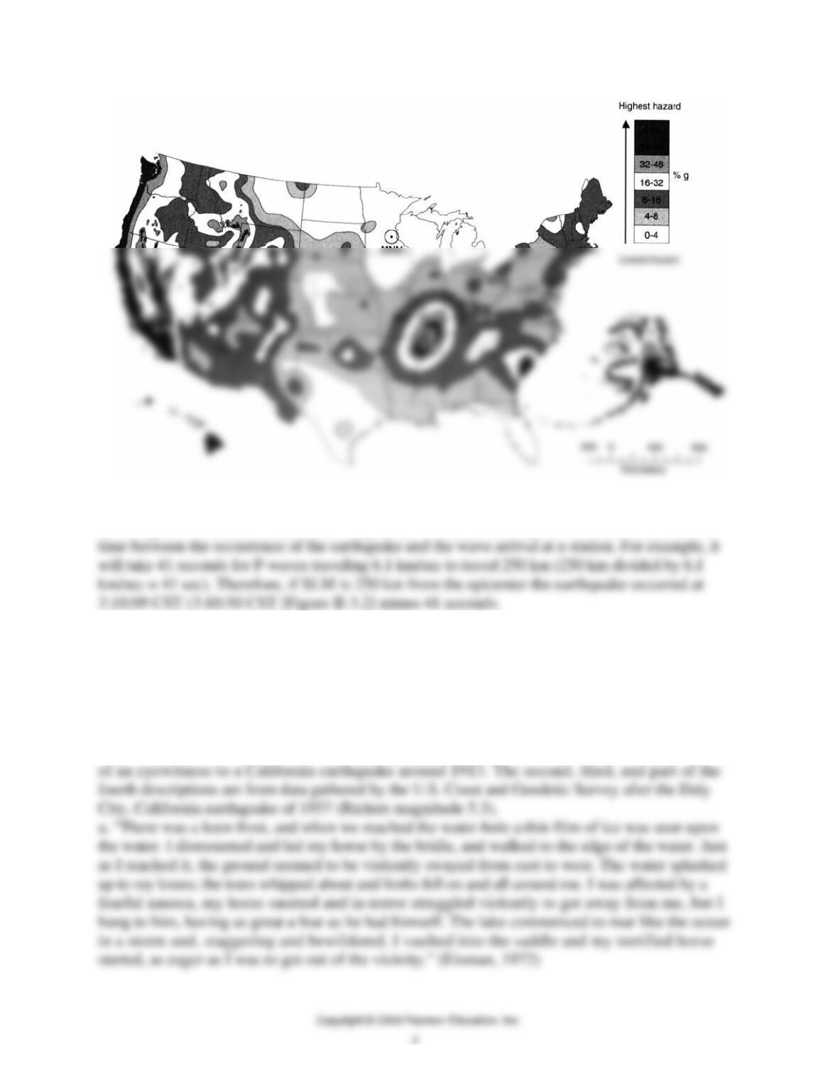
1. Which areas of the country have the lowest hazard from earthquake shaking (where 4% g, or
less, peak acceleration is expected)?
2. If damage to older (pre-1965) structures can be expected with horizontal accelerations of 10%
g or more, which areas of your home state are:
a. at some risk?
b. at greatest risk?
c. what is your home state?
3. What three or four regions of the country have the highest accelerations?
4. What geologic processes, other than shaking and fault displacement, could produce a hazard in
an earthquake? List two.
5. The geologic material on which a building rests plays a role in the type of shaking that occurs
during an earthquake. Weak materials amplify the shaking. Which of the following foundation
materials would most likely result in less shaking and a safer building? (Circle one.)
6. If the Internet is available, now or after class, determine and list (places and magnitudes)

7. The Mississippi Valley is indicated as a high-risk area because of earthquake activity that is
associated with stress within the continental lithospheric plate. Consider the types of plate
margins in the plate tectonics model to answer the following questions. (See a geology text for
basic details on plate margins.)
a. What is the tectonic explanation for the major shaking hazard in southern California?
QUESTIONS 6, PART B
Fault Diagrams
1. The freshly exposed cliff of bedrock or regolith along a fault line is known as a fault scarp.
2. Following an earthquake, the horizontal distance between two utility poles on opposite sides
of a fault trace (not a strike-slip fault) had increased. Are the regolith (soils) and bedrock in this
area in a region of compression (squeezing together) or tension (pulling apart)? Explain your
3. Sketch two utility poles on Figure 6.6a, placing one on each side of the fault. Use fault
diagrams Figure 6.6b and c, and determine if the relative motion of the fault blocks in Question 2
indicates that it is a normal fault or reverse fault. Explain your reasoning.
Normal fault (not strike slip).
4. What geological features can be used to identify the location of the fault? Outline the fault
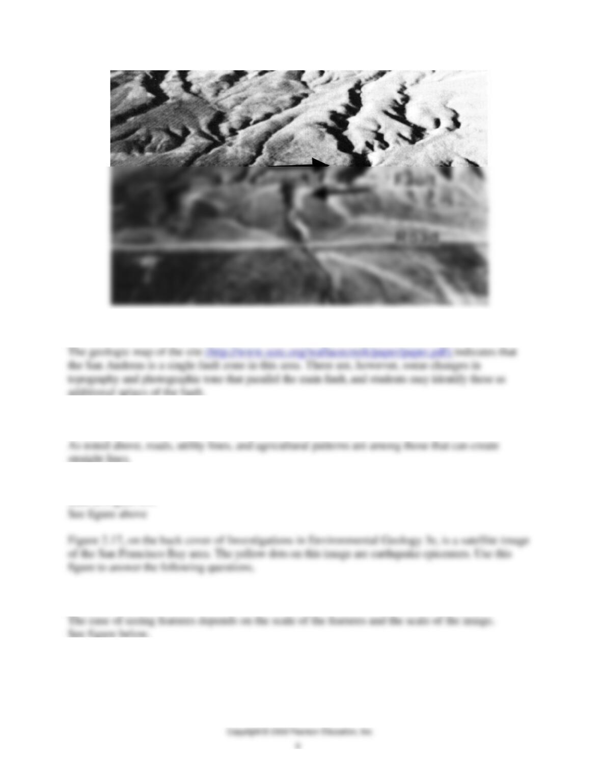
5. Does the fault zone consist of a single fracture or several parallel fractures? What is your
evidence?
6. In addition to faults, what other natural or human-made features can create straight lines in
topography? Are any of these features present in this photograph?
7. Indicate the direction of movement along the fault by drawing arrows on either side of the
fault in Figure 6.9.
8. Which features of strike-slip faults shown on Figure 6.7 can be seen easily on the satellite
image? Why are some features easier than other features to see on the image?
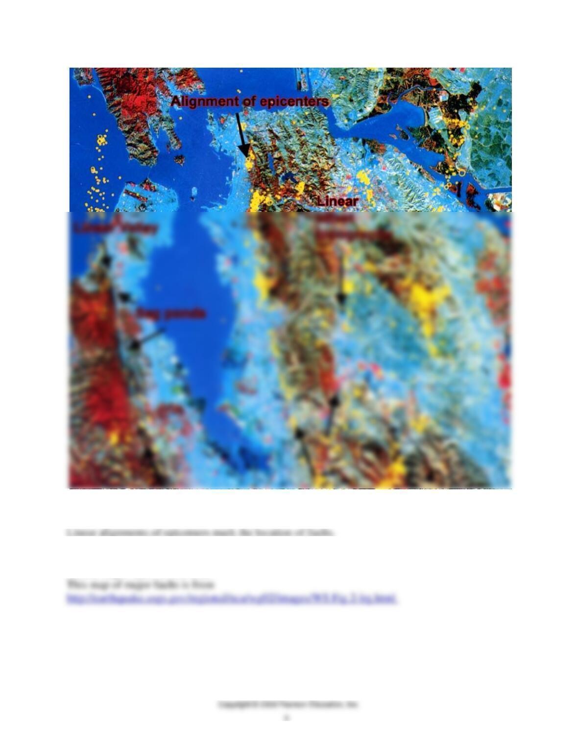
9. How do the locations of earthquake epicenters help you determine geographic features that are
related to faults?
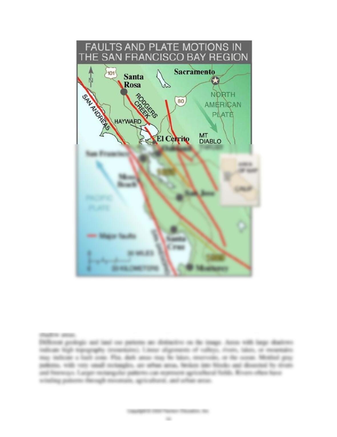
10. Mark on the back cover (Figure 2.17) or on a tracing such as Figure 2.18, the traces of
several major faults in this area.
Study the radar image of southern California in Figure 6.10. This image was made from an
airplane that bounced radar waves off the earth. The radar is able to penetrate vegetation and
clouds, so the image is very clear. The surface of the land is shown as if the sun lighted it, with
bright slopes facing the sun and dark areas of shadow. Of course, in a radar image it is not
sunlight but is the location of the airplane sending out the radar that creates the bright and
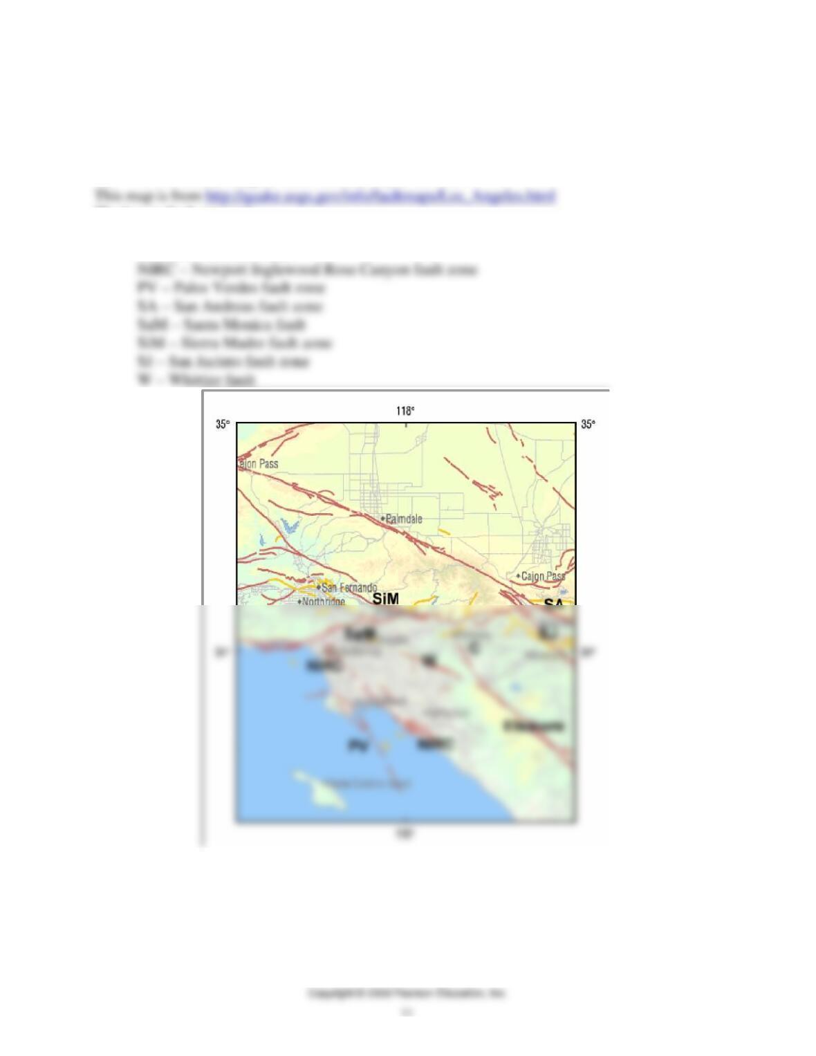
11. What evidence of faults do you see on the radar
image? Linear traces of topography (straight lines that are not
roads).
12. Draw on the image all the fault traces you can find.
The key to fault names is:
C – Chino fault
Elsinore – Elsinore fault
13. Use the Web, or material provided by the instructor, to label faults including the Elsinore and
San Andreas on Figure 6.10.
See map above
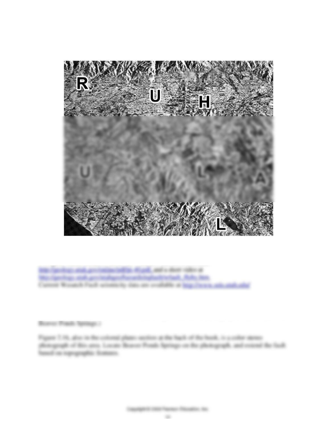
14. Find and label an example of the following: agriculture pattern (A), urban region (U), major
highway (H), lake (L), and river (R).
See the cropped and edited version of the radar image below.
Wasatch Fault
Two good online resources about the Wasatch Fault are a brochure:
15. Study the map of the Draper, Utah, quadrangle (Figure 6.11 in the colored plates section of
this book) and mark on the map the location of the Wasatch Fault along the mountain front.
(Hint: Refer to Figure 6.8 for features found along normal faults, and begin your identification at
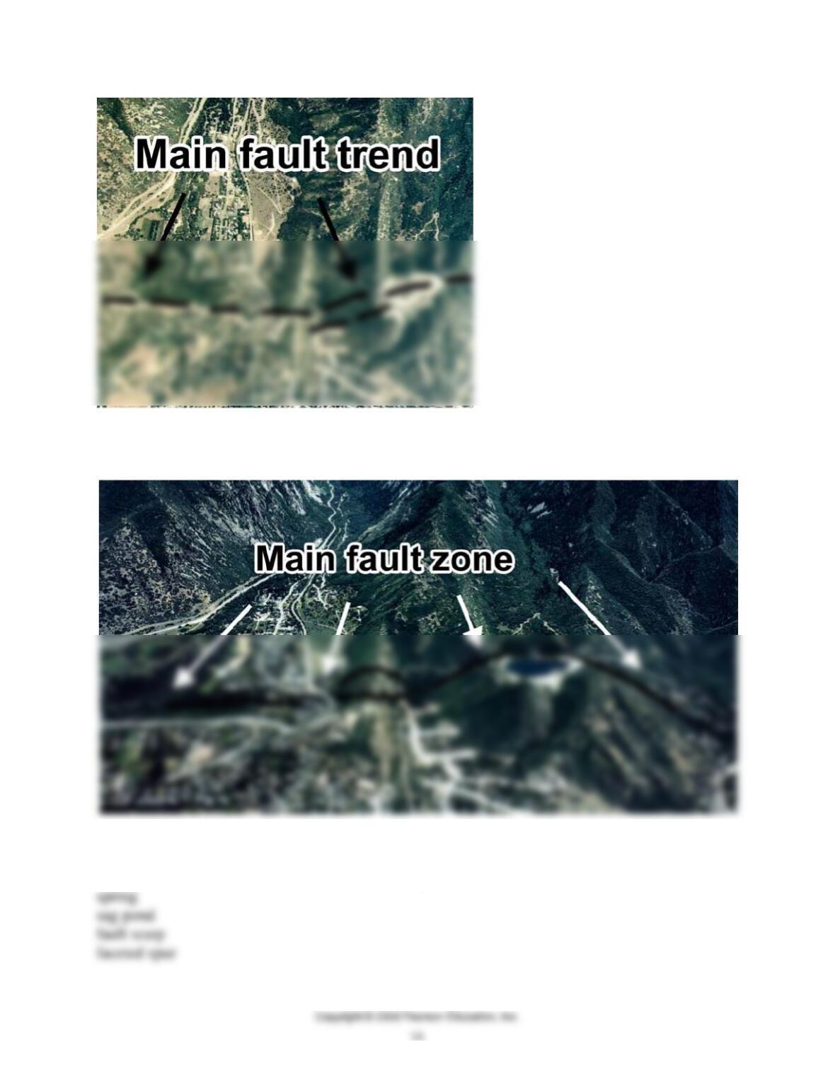
Faults can also be seen on color oblique photographs. Use Figure 6.12 and identify on it the fault
scarp and extend trace of the fault both north and south.
16. Using information on normal faults from Figures 6.6, 6.7, and 6.8, review the photographs of
the site (Figures 2.16 and 6.12) and the map (Figure 6.11), and describe the location and
appearance of at least one of each of the following features of a normal fault:

See maps above for locations.
17. In the San Andreas Fault example (questions 4 and 5 above), lateral stream offset was an
important clue to movement along the fault. Follow the traces of streams in Figure 6.11 as they
flow west from the mountains to the valley. Is there any offset of streams where they cross the
fault(s)? Why or why not?
18. Can you tell from the map (Figure 6.11) which side of the fault has moved up and which side
has moved down? Describe your evidence. What additional kinds of information might be
helpful in determining the movement along the fault?
Of course, the mountainside has moved up. Individual fault splays, however, may create local
19. Look at the aerial photograph in Figure 6.13. Identify on this figure any linear zones you see
that might be faults, being careful to avoid roads and property lines that are marked by cut
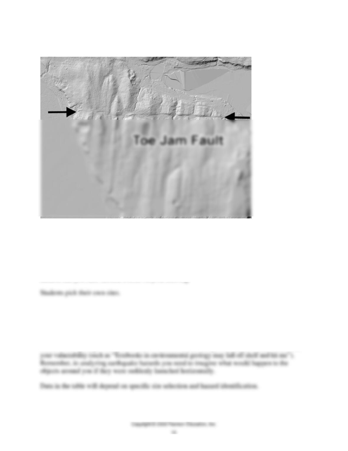
20. Figure 6.14 is a LIDAR image of the same area, processed to remove the forest from the
image. Mark on this figure any traces of faults that you see. Compare the trace of the fault with
the drawings in Figures 6.7 and 6.8. What are the surface features that you see along the fault?
What kind of fault movement and offset is most likely here? (Circle one.) Normal, Reverse,
Strike slip?
This is the Toe Jam strand of the Seattle Fault (we kid you not; it is named after the local
trenches across 2-to-3-m-high scarps suggests postglacial deformation above a north-
dipping, blind reverse fault.”
QUESTIONS 6, PART C
1. Select a site that you frequently use. Make a sketch of this room on the graph paper provided
in Figure 6.16. The choice of site is up to you. It could be a dorm room, a bedroom at home, a
place where you work, a place where you study, or some other room or facility. You may do a
map view or an elevation, but there is no need to do both. Identify and label the nonstructural
hazards that you find. Include a scale on your drawing.
2. The list in Table 6.5 identifies some of the nonstructural hazards that you may encounter in
your search. This list is not intended to be comprehensive; there are undoubtedly some missing
hazards. Space is left at the bottom of the list for you to add other hazards that you discover.
Identify the room and building in the table title. Then identify all hazards in the room that you
select. In the space provided, make brief comments about the specific nature of each hazard and

PART D. EARTHQUAKE PREPARATION AND HAZARD REDUCTION
Use a separate sheet of paper for answers to Questions 1 and 2.
1. Assume that you have three different amounts to spend on earthquake preparation for you or
2. Imagine that an earthquake occurs while you are in a class. What would you want from your
educational institution immediately? What would you want over the next few days? How soon
would you want to be back in class? Develop a separate list of items that you believe your
educational institution should be ready to provide or situations that it should be prepared to deal
with after an earthquake. Divide your list into two sections, with the first section itemizing needs
during the first 72 hours, and the second section listing longer-term considerations. Who do you
contact at your school to determine which preparations on your list have been made and which
are still needed?
Students should note that they would like their schools to be back in session fairly rapidly.