Section 4.2 Solving Systems of Linear Equations by the Substitution Method
39.
0.7 0.1 0.6
0.8 0.3 0.8
xy
xy
Multiply both sides of both equations by 10.
76
83 8
xy
xy
Solve the first equation for y.
76
xy
40.
1.25 0.01 4.5
0.5 0.02 1
xy
xy
Multiply both sides of both equations by 100.
125 1 450
50 2 100
xy
xy
Solve the first equation for y.
125 1 450
xy
Back-substitute.
125 450 125 4 450
500 450 50
yx
The solution set is
4,50 .
41. a. Substitute
0.001 3x
for p in the first equation.
0.002 6
0.001 3 0.002 6
0.001 3 0.002 6
0.002 0.001 3 0.002 0.002 6
p
px
xx
xx
xx xx
b. If unleaded premium gasoline is sold for $4 per
gallon, there will be a demand for 1000 gallons
per day and 1000 gallons will be supplied per
day.
42. a. Substitute
0.5 5x
for y in the first equation.
0.5 105
0.5 5 0.5 105
y
yx
xx
$0.50
b. If cookies are sold for $0.50 per package, there
will be a demand for 110 million packages and
bakers will supply 110 million packages per
Chapter 4 Systems of Linear Equations
49. does not make sense; Explanations will vary.
Sample explanation: Solving for x in the second
equation will allow us to avoid fractions.
53. true
54. false; Changes to make the statement true will vary.
A sample change is: The graphing method allows us
to visualize solutions.
56.
3
26
311
xyz
xyz
xyz
First substitute 3yzfor x in the second
equation.
26
xyz
Now substitute 3yz in the third equation of the
given system.
311
xyz
Substitute
12 3z
in the last equation.
94 2 11
9 4 12 3 2 11
yz
zz
33351xyz
Thus, x = 1, y = −3, and z = 5.
57.
3
52 7
ymx
xy
257
57
22
yx
yx
The system will be inconsistent if the graphs of the
two equations have the same slope and different y-
intercepts. The y-intercepts are different. Therefore,
the system will be inconsistent if
5
m
.
4612
4(0) 6 12
612
xy
y
y
Section 4.3 Solving Systems of Linear Equations by the Addition Method
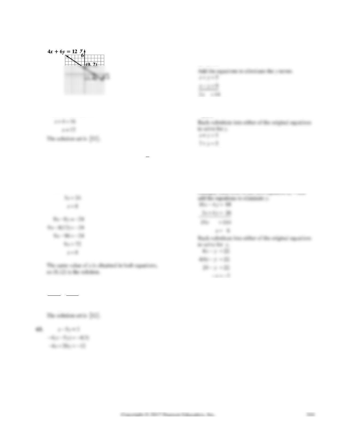
Draw a line through (3,0), (0, 2), and (−3, 4).
59.
412533
442539
xx
xx
60. The integers in the given set are −73, 0, and
33.
1
61.
32 48
32(12)48
32448
xy
x
x
62.
14 168
14 168
14 14
12
y
y
y
4.3 Check Points
1.
5
9
xy
xy
Now solve for x.
214
x
2
y
The solution set is
7, 2 .
2.
422
34 26
xy
xy
2
y
The solution set is
6, 2 .
Chapter 4 Systems of Linear Equations
3.
45 3
23 7
xy
xy
Multiply each term of the second equation by –2
and add the equations to eliminate x.
45 3
xy
4.
293
483
xy
yx
Rewrite each equation in the form .
A
xByC
23 9
xy
Back-substitution of
60
17
to find y would cause
cumbersome arithmetic.
Instead, use the system that is in the form
A
xByC
to eliminate x and find y.
23 9
xy
5.
24
36 13
xy
xy
Multiply the first equation by −3.
36 12
xy
The true statement indicates that the system has
infinitely many solutions.
The solution set is
,57xy x y
or
, 3 15 21 .xy x y
4.3 Exercise Set
1.
3
11
xy
xy
Add the equations to eliminate the y-terms.
Section 4.3 Solving Systems of Linear Equations by the Addition Method
2.
6
2
xy
xy
Add the equations to eliminate the y-terms.
6xy
4
y
The solution set is
2, 4 .
3.
23 6xy
23 6xy
412
3
x
x
4.
32 14xy
32 10xy
624
4
x
x
Back-substitute into either of the original equations
to solve for y.
5. 27xy
318xy
525
y
6. 2 2xy
23 6xy
28
4
y
y
Back-substitute into either of the original equations
to solve for x.
2 2
xy
to solve for x.
5114
515
3
x
x
x
The solution set is
3,1 .
Chapter 4 Systems of Linear Equations
9.
3 7
25 1
xy
xy
Multiply each term of the first equation by 5 and
add the equations to eliminate y.
10. 311
2513
xy
xy
Multiply first equation by 5 and add.
15 5 55
2513
xy
xy
x
11. 34
45 2
xy
xy
Multiply each term of the first equation by −4 and
add the equations to eliminate x.
Back-substitute into either of the original equations
to solve for x.
34
32 4
xy
x
to solve for x.
21
22 1
41
3
xy
x
x
x
The solution set is
3, 2 .
to solve for y.
213
27 13
14 13
xy
y
y
Section 4.3 Solving Systems of Linear Equations by the Addition Method
14. 25 1
37
xy
xy
Multiply the second equation by 5 and add.
25 1
xy
15. 314 6
5710
xy
xy
Multiply each term of the second equation by 2 and
add the equations to eliminate y.
314 6
xy
The solution set is
2,0 .
16. 54 19
32 7
xy
xy
Multiply the second equation by 2 and add.
Back-substitute into either of the original equations
to solve for y.
32 7
33 2 7
xy
y
17x 17
x = 1
Back-substitute into either of the original equations
to solve for y.
23 4
xy
35 140
4
y
y
Back-substitute into either of the original equations
to solve for x.
Chapter 4 Systems of Linear Equations
19. 32 1
27 9
xy
xy
Multiply the first equation by 2 and the second
equation by 3.
64 2xy
A
20. 53 27
7213
xy
xy
Multiply the first equation by 2.
Multiply the second equation by 3.
10 6 54xy
21. 327
5213
xy
xy
Rewrite each equation in the form .
A
xByC
32 7
52 13
xy
xy
Back-substitute into either of the original equations
to solve for y.
327
33 2 7
xy
y
9 25xy
92 4xy
321
7
y
y
Back-substitute into either of the original equations
612 6
xy
Rewrite the first equation in the form .
A
xByC
23 4xy
Multiply the first equation by 3 and add to
eliminate x.
69 12xy
612 6xy
Section 4.3 Solving Systems of Linear Equations by the Addition Method
24. 548
37 14
xy
xy
Rewrite the first equation in the form .
A
xByC
54 8
37 14
xy
xy
25. 23
44 1
xy
xy
Multiply the first equation by 4 and add to
eliminate y.
84 12xy
A
6
The solution set is
11 7
,.
12 6
26.
322
45 21
xy
xy
Multiply the first equation by 5.
15 5 110xy
45 21xy
The solution set is
89 151
,.
19 19
27.
452
23 4
xy
xy
Rewrite the first equation in the form
16 23
23
16
x
x
The solution set is
23 3
,.
16 8
Chapter 4 Systems of Linear Equations
28.
341
431
xy
xy
Rewrite the first equation in the form
,
A
xByC
and multiply the second equation
by −3.
12 16 4
A
xy
34 1
431
xy
xy
To eliminate y, multiply the first of these equations
by 3 and the second by 4.
9 12 3
xy
29.
31
32
xy
xy
Multiply the first equation by −1.
31
xy
30.
49 2
49 2
0 4, false
xy
xy
31. 32xy
39 6xy
Multiply the first equation by −3.
39 6xy
39 6xy
42 2
42 2
0 0, true
xy
xy
The true statement indicates that the system has
14 6 8xy
14 6 7xy
0 = 1, false
The false statement indicates that the system is
Multiply the second equation by −2.
612 15
612 12
0 3, false
xy
xy
35.
52
31
xy
xy
Multiply the second equation by −1.
52xy
31xy
36.
25 1
21
xy
xy
Multiply the first equation by −1.
251
2 1
xy
xy
37.
53
26 10
xy
xy
The true statement indicates that the system has
infinitely many solutions.
The solution set is
,53xy x y
or
,26 10.xy x y
The solution set is
,4 368xy x y
or
,36 27.xy x y
39.
43 0
3310
xy
xy
Rewrite both equations.
3
The solution set is
1,1 .
3
Chapter 4 Systems of Linear Equations
40.
22 3 0
73232
xy
xy
Rewrite each equation in the form .
A
xByC
Now solve the system formed by the two rewritten
equations.
46 0
76 11
xy
xy
41.
11
1
57
xy
xy
Multiply the second equation by the LCD, 35, to
clear fractions.
35 35 1
57
75 35
xy
xy
42.
3
1
97
xy
xy
Now solve the system
3
79 63
xy
xy
Multiply the first equation by −7 and add the result
to the second equation.
43.
5
21
5
xy
xy
Multiply both equations by 5 to clear fractions.
45 5xy
25 5
xy
60
0
x
x
Section 4.3 Solving Systems of Linear Equations by the Addition Method
44.
3
3
1
24
xy
xy
To clear fractions, multiply the first equation by 3
and the second equation by 4 to obtain the system.
39
xy
45.
32 8
2
xy
xy
The substitution method is a good choice because
the second equation is already solved for x.
Substitute −2y for x in the first equation
46.
210
3
xy
yx
The substitution method is a good choice because
Back-substitute −10 for x into the second equation
of the system.
3
310 30
yx
y
The solution set is
10, 30 .
47.
32 3
xy
33
1
x
x
The solution set is
1, 3 .
48.
27 17
xy
2717
27117
2717
xy
x
x
49.
32 6
3
xy
y
The substitution method is a good choice because
the second equation is already solved for y.
Substitute 3 for y in the first equation.
32 6
xy
50.
23 7
2
xy
x
The substitution method is a good choice because
the second equation is already solved for x.
Substitute 2 for x in the first equation.
23 7
xy
51.
21
23
yx
yx
The substitution method is a good choice, because
both equations are already solved for y. Substitute
A
52.
24
21
yx
yx
The substitution method is a good choice, because
both equations are already solved for y.
Substitute
24
x
for y in the second equation.
2421
xx
The addition method is a good choice since the
equations can easily be simplified to give equations
of the form .
A
xByC
24 6
xy
36 90
36 9
xy
xy
Solve the resulting system.
The solution set is
,2 2 6
xy x y
or
,3 2 30.
xy x y
54.
241
xy x
Section 4.3 Solving Systems of Linear Equations by the Addition Method
Now solve the system formed by the two rewritten
equations.
22 1
xy
2
55.
32
29 24
yx
xy
The substitution method is a good choice because
56.
45
58 20
yx
xy
The addition method is a good choice because the
Multiply the second equation by −1, and the result
to the rewritten equation.
54 0
xy
57.
514
44
xy
xy
Add the equations.
514
xy
5
x
Back-substitute into the first equation of the original
system.
32 11
3(5) 2 11
xy
y
Chapter 4 Systems of Linear Equations
59.
43 0
7
xy
xy
Multiply the second equation by 3 and then add the
equations.
60.
36 15
2
xy
xy
Multiply the second equation by 6 and then add the
equations.
36 15
xy
61.
341
55
3
1
48
xy
xy
Multiply the first equation by 5 and the second
Multiply the first equation by 3 and the second
equation by 4.
912 15
812 32
xy
xy
62.
2
32 3
24
33
xy
xy
2
x
Back-substitute 2 for x in the equation and solve for
y.
23 4
22 3 4
xy
y
Section 4.3 Solving Systems of Linear Equations by the Addition Method
63.
517 17
61551
xy
xy
Simplify both equations.
51717
557 77
xy
xy
57 5
65 6
xy
xy
Multiply the first equation by −6 and the second
equation by 5, and solve by addition.
30 42 30
30 25 30
17 0
xy
xy
y
64.
65 3
3451
xxy x
xy y y
Simplify both equations.
65 3
xxy x
Solve the rewritten system.
2515
34 5
xy
xy
Multiply the first equation by -3 and the second
equation by 2, and solve by addition.
615 45
xy
65. 0.4 2.2
0.5 1.2 0.3
xy
xy
Multiply the first equation by 1.2 and solve by
addition.
0.48 1.2 2.64
0.50 1.2 0.30
xy
xy
66. 1.25 1.5 2
3.5 1.75 10.5
xy
xy
Multiply the first equation by –2.8 and solve by
addition.
Chapter 4 Systems of Linear Equations
Back-substitute 2 for y to find x.
1.25 1.5 2
xy
67. 8
23
211
23
xy
xy
Simplify the first equation.
8
23
xy
When simplified, the equations are the same. This
means that the system is dependent and there are an
infinite number of solutions.
68. 8
24
35
24
xy
xy
Simplify the first equation.
Simplify the second equation.
35
21
21
xy
xy
yx
When simplified, the both equations have the same
slope, but different y-intercepts. This means that
the system is inconsistent and there are no solutions.
The solution set is
.
69. 0.45 0.8
xy
2.7 0.8
3.5
y
y
The solution is (6, 3.5). This means that in week 6,
b. In 2015 both will receive 50%.
c. 2112
288
xy
xy
Add the equations.
Section 4.3 Solving Systems of Linear Equations by the Addition Method
Back-substitute 50 for y and solve for x.
2112
xy
d. reasonably well
71. – 75. Answers will vary.
76. makes sense
77. does not make sense; Explanations will vary.
Sample explanation: The addition method does not
involve graphing.
81. false; Changes to make the statement true will vary.
A sample change is: If (2, 2) satisfies
22Ax y
and 210,xBythen A and B can be
found by substitution.
Find A.
22
Ax y
83. false; Changes to make the statement true will vary.
A sample change is: After these multiplications, the
2
xxba
xb a
xab
xab
Back-substitute ab for x to find y.
2
2
yxb
yabb
2
A
37
35 2 7
15 2 7
28
xBy
B
B
B
Chapter 4 Systems of Linear Equations
88. 29,700 150 5000 1100
29,700 950 5000
950 24,700
26
xx
x
x
x
The solution set is {26}.
89. a. 28
6
xy
xy
Mid-Chapter Check Point – Chapter 4
1.
32 6
2 4
xy
xy
x
y
-4 -2 2 4
-4
-2
2
4
0
The lines intersect at (2, 0).
The solution set is
2,0 .
3. 21
6312
yx
xy
x
y
-4 -2 2 4
-4
-2
2
4
0
373571578yx
The solution set is
5,8 .
5.
65 7
37 13
xy
xy
Multiply the second equation by −2 and add to
eliminate x.
6 5 7
614 26
19 19
1
xy
xy
y
y
Back-substitute −1 for y and solve for x.
65 7
xy