Chapter 3
Linear Equations in Two Variables
3.1 Check Points
1.
b.
39
23(3) 9
29 9
11 9, false
xy
(2,3) is not a solution.
4.
32 (,)
23(2)242,4
13(1)211,1
xyx xy
y
y
5.
2(,)
22(2)42,4
12(1)21,2
xyx xy
y
y
6.
22 (,)
22(2)262,6
12(1)241,4
xyx xy
y
y
1
2
1
2
1
2
1
2
2(2)212,1
0(0)220,2
2(2)232,3
4(4)244,4
y
y
y
y
51.4(5)18(5,8)
10 1.4(10) 1 15 (10,15)
15 1.4(15) 1 22 (15,22)
D
D
D
2015.
d. 1.4 1
Dn
3.1 Concept and Vocabulary Check
1. x-axis
2. y-axis
3. origin
3.1 Exercise Set
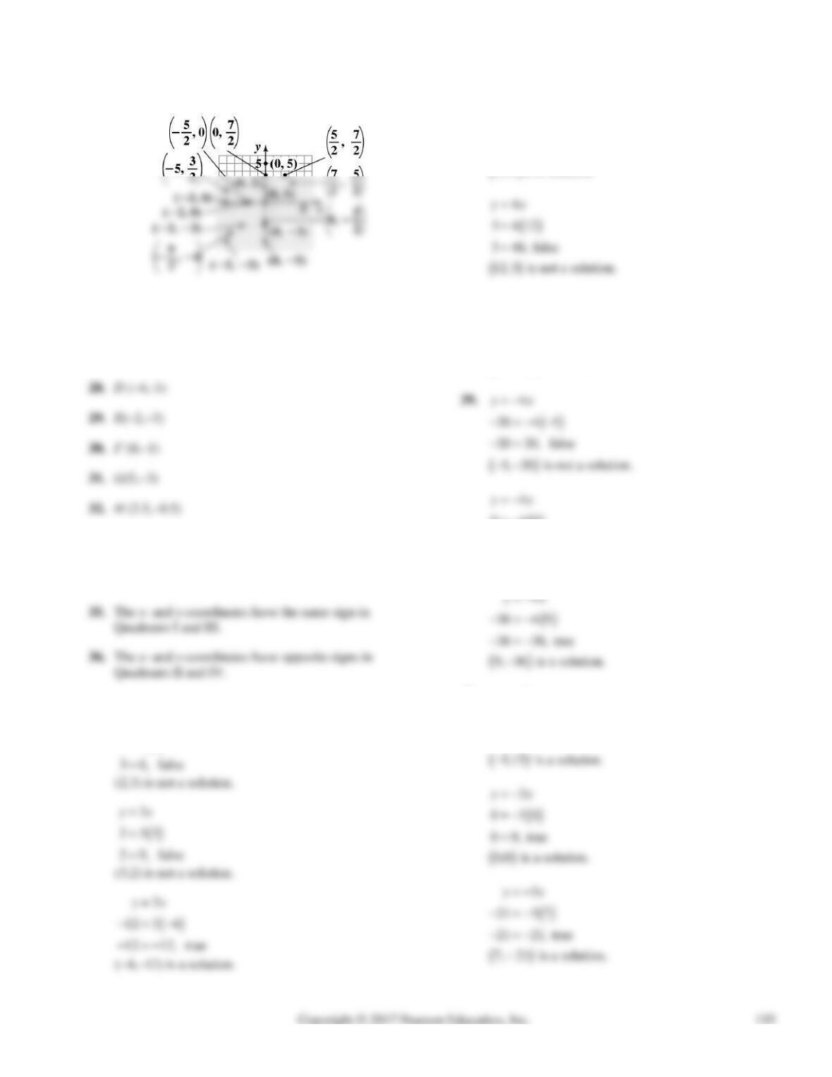
1. Quadrant I
5. Quadrant III
7. Quadrant IV
Section 3.1 Graphing Linear Equations in Two Variables
9. – 24.
25. A (5,2)
26. B (-2,4)
27. C (−6,5)
33. The y-coordinates are positive in Quadrants I and II.
34. The x–coordinates are negative in Quadrants II and
III.
37. 3yx
3
332
yx
38.
4
12 4 3
12 12, true
yx
3,12 is a solution.
4
20 4 5
20 20, true
yx
5, 20 is a solution.
040
00, true
0,0 is a solution.
40.
3
15 3 5
15 15, true
yx
Chapter 3 Linear Equations in Two Variables
41.
26
620 6
66, true
yx
0,6 is a solution.
42.
84
0848
8832
8 24, false
yx
8,0 is not a solution.
43.
35 15
35 56 15
15 30 15
15 15, true
xy
35 15
310 5 3 15
30 15 15
15 15, true
xy
20 30 0
50 0, false
10,6 is not a solution.
25 0
25 50 0
xy
1 1 0
2 0, false
1
1, is not a solution.
3
Section 3.1 Graphing Linear Equations in Two Variables
46.
50
050 0
00 0
xy
2 0, false
1
1, is not a solution.
5
47.
40
44 0
00, true
x
4,7 is a solution.
48.
20
22 0
40, false
y
20
22 0
0 0, true
y
0, 2 is a solution.
50.
14 ( , )
2 14 2 28 2, 28
1141141,14
014000,0
xyx xy
y
y
y
52.
20 ( , )
2 20 2 40 2, 40
1 20 1 20 1,20
xyx xy
y
y
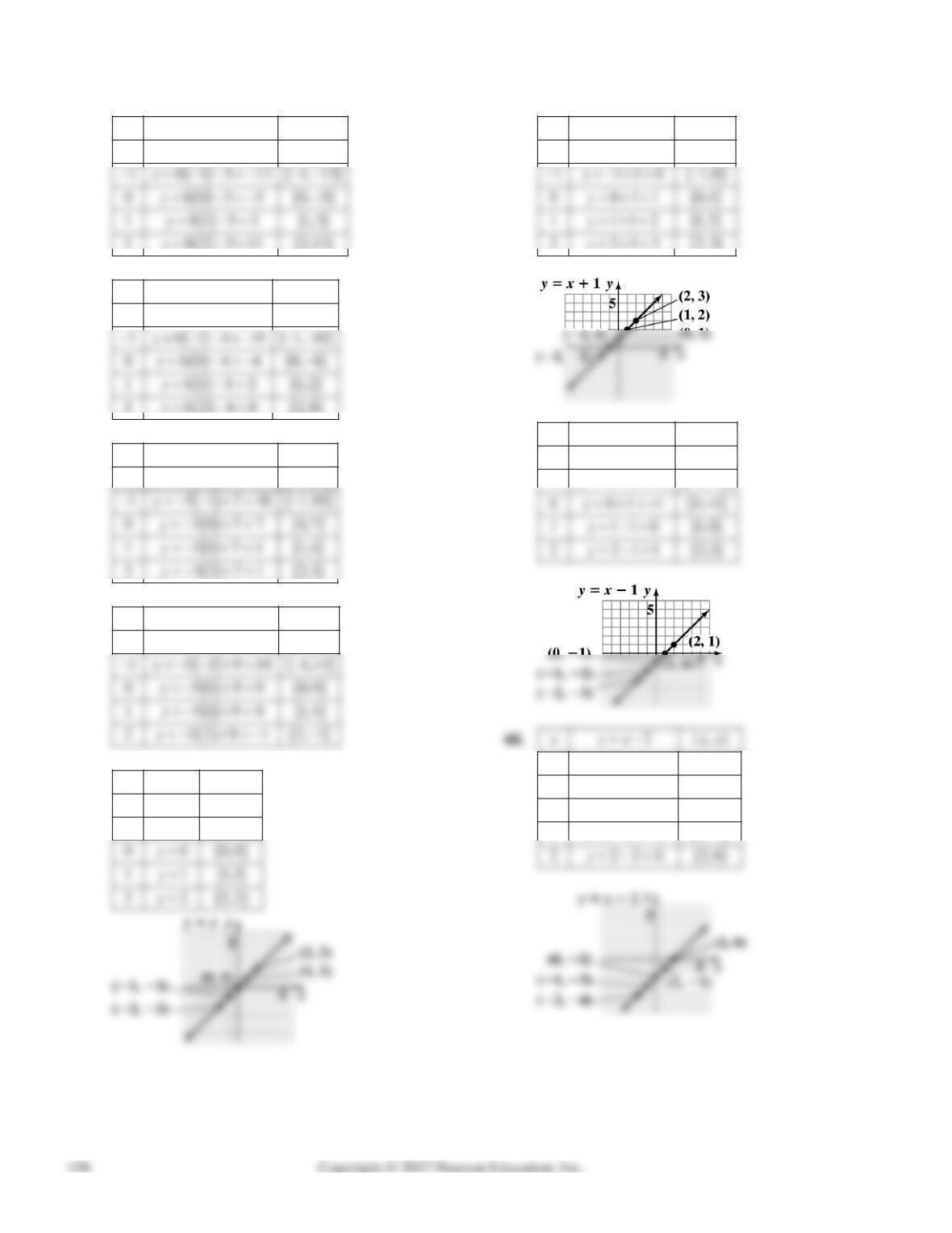
Chapter 3 Linear Equations in Two Variables
53.
85 (,)
2 8 2 5 21 2, 21
xyx xy
y
54.
62 4 16 2,16
64 (,)
2
y
xyx xy
55.
37 (,)
2 3 2 7 13 2,13
xyx xy
y
56.
59 (,)
2 5 2 9 19 2,19
xyx xy
y
57.
(, )
222,2
111,1
xyx xy
y
y
58.
1(,)
22112,1
xyx xy
y
59.
1(,)
22132,3
11121,2
xyx xy
y
y
22242,4
11231,3
00220,2
11211,1
y
y
y
y
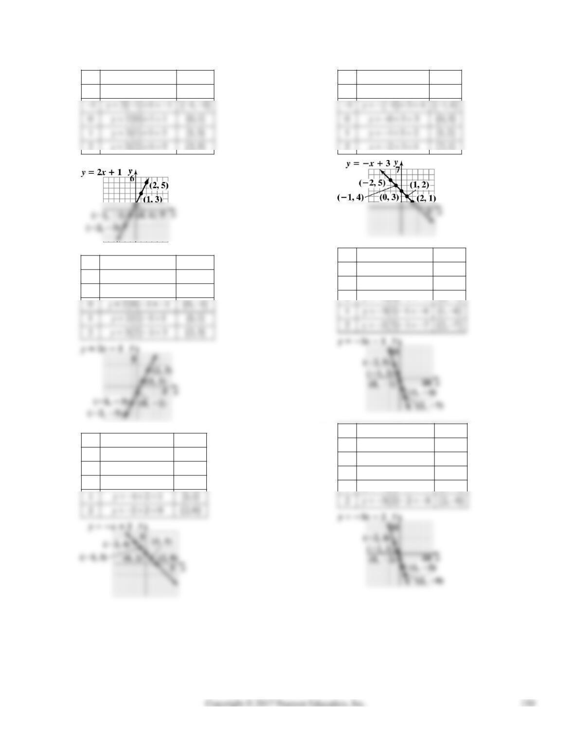
Section 3.1 Graphing Linear Equations in Two Variables
61.
21 (,)
222132,3
xyx xy
y
62.
21 (,)
222152,5
121131,3
xyx xy
y
y
63.
2(,)
22242,4
11231,3
00220,2
xyx xy
y
y
y
64.
3(,)
22352,5
xyx xy
y
65.
31 (,)
232152,5
131121,2
xyx xy
y
y
66.
32 (,)
232242,4
131211,1
030220,2
131251,5
xyx xy
y
y
y
y
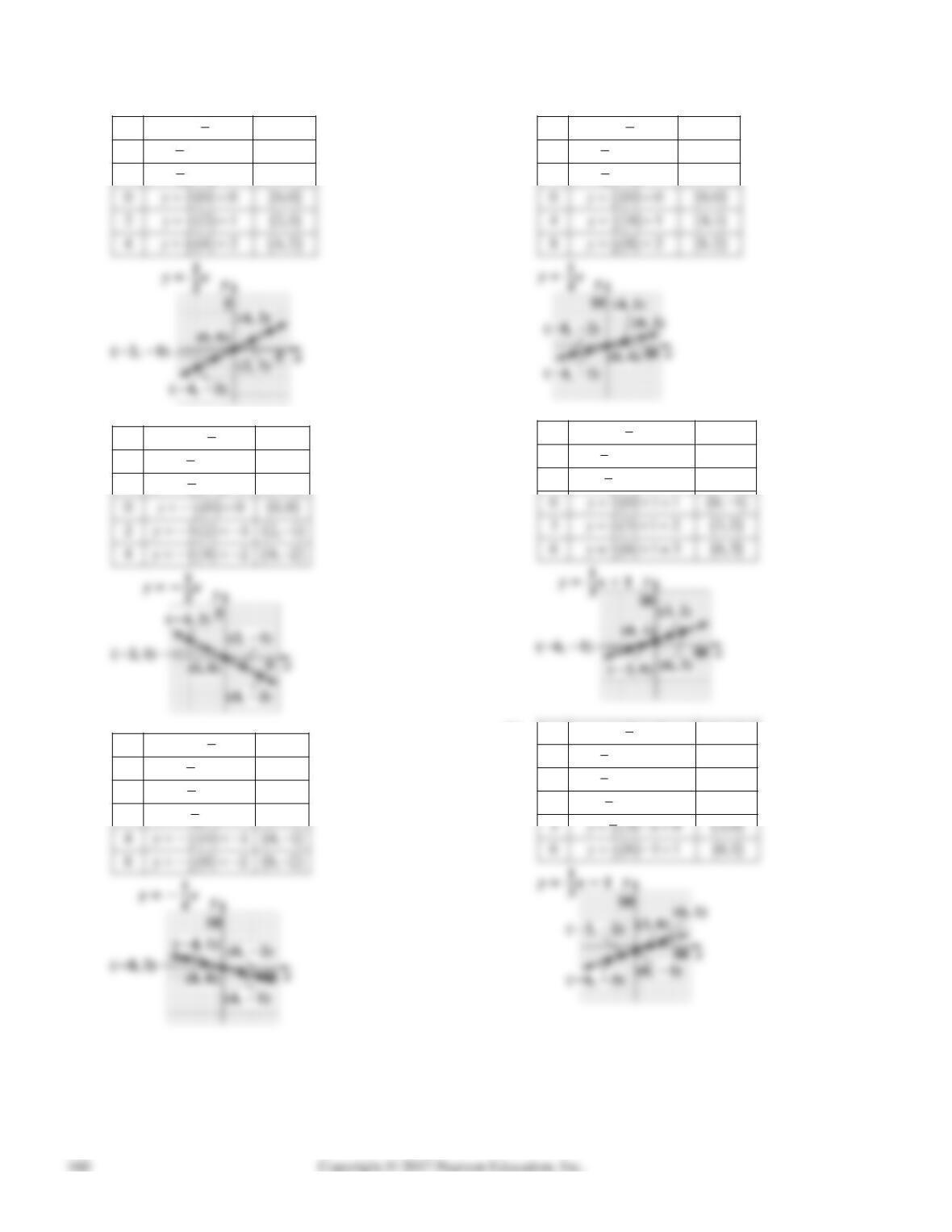
Chapter 3 Linear Equations in Two Variables
67.
1
2
1
2
1
2
(, )
4424,2
2212,1
xyx xy
y
y
68.
1
2
1
2
1
(, )
4424,2
2212,1
xyx xy
y
y
69.
1
4
1
4
1
4
1
4
(, )
8828,2
4414,1
0000,0
xyx xy
y
y
y
70.
1
4
1
4
1
4
(, )
8828,2
4414,1
xyx xy
y
y
71.
1
3
1
3
1
3
1(,)
66116,1
33103,0
xyx xy
y
y
72.
1
3
1
3
1
3
1
3
1
1(,)
66136,3
33123,2
00110,1
xyx xy
y
y
y
Section 3.1 Graphing Linear Equations in Two Variables
73.
3
2
3
2
3
2
3
1(,)
44174,7
22142,4
00110,1
xyx xy
y
y
y
74.
3
2
3
2
3
2
3
2(,)
44284,8
22252,5
00220,2
xyx xy
y
y
y
75.
5
2
5
2
5
2
5
2
1(,)
44194,9
22142,4
00110,1
xyx xy
y
y
y
76.
5
2
5
2
5
2
5
1(,)
441114,11
22162,6
00110,1
xyx xy
y
y
y
77.
1
2
1
2
1
2
1
(, )
443.54,3.5
221.52,1.5
xyx xy
y
y
78.
1
2
(, )
xyx xy
Chapter 3 Linear Equations in Two Variables
79.
04 (,)
606446,4
303443,4
000440,4
xyx xy
y
y
y
80. 3, or 0 3yyx
03 (,)
707337,3
404334,3
000330,3
xyx xy
y
y
y
81. 3yx
82. 4yx
83. 25yx
85. a. 8 6 14.50xy
b.
8 6 0.75 14.50
8 4.50 14.50
x
x
312.00
4.00
x
x
An orange tree costs $4.00.
87. The coordinates of point A are (2,7). When the
football is 2 yards from the quarterback, its height is
7 feet.
88. The coordinates of point B are (28,7). When the
football is 28 yards from the quarterback, its height
is 7 feet.
Section 3.1 Graphing Linear Equations in Two Variables
92. The football’s height is 5 feet when it is caught by
93. a.
2.4 31 ( , )
02.4(0)3131(0,31)
52.4(5)3143(5,43)
nSn nS
S
S
b. Graph of formula:
c. According to the graph in part (b), the
percentage is approximately 74%.
d.
2.4 31
Sn
2018.
94. a.
1.7 45 ( , )
01.7(0)4545(0,45)
5 1.7(5) 45 36.5 (5,36.5)
nQn nQ
Q
Q
b. Graph formula:
c. According to the graph in part (b), the
percentage is approximately 14%.
d.
1.7 45
Qn
103. makes sense
104. makes sense
107. false; Changes to make the statement true will vary.
A sample change is: The lines are not parallel as
they both contain the point (1,2).
108. true
Chapter 3 Linear Equations in Two Variables
111. a.
13
1, , 2,1 , 3, , 4, 2
22
b. In order for the resulting graph to be a mirror-
image reflection about the y-axis of the graph in
c. In order for the resulting graph to be a mirror-
image reflection about the x-axis of the graph in
part (a), the sign of each y-coordinate should be
d. In order for the resulting graph to be a straight-
line extension of the graph in part (a), the signs
of both coordinates of each ordered pair should
be changed:
112. 21yx
113. Answers will vary depending upon the points
chosen. One example is shown here.
116. Answers will vary.
Section 3.2 Graphing Linear Equations Using Intercepts
117.
354237
xx
358127
3585
xx
xx
118.
31 2 5 28 31 10 28
39 28
27 28 1
119.
1 for
3
VAhh
1
3
VAh
120.
34 24
34(0)24
324
xy
x
x
122.
20
02 0
20
xy
y
y
3.2 Check Points
1. a. The graph crosses the x-axis at (–3,0). Thus, the
x-intercept is –3.
y-intercept is 0.
2. To find the x-intercept, let y = 0 and solve for x.
4312
43(0)12
412
3
xy
x
x
x
The x-intercept is 3.
4. Find the x-intercept. Let y = 0 and solve for x.
23 6
23(0)6
26
3
xy
x
x
x
Chapter 3 Linear Equations in Two Variables
Find a checkpoint. For example, let x = 1 and solve
for y.
23 6
2(1) 3 6
xy
y
5. Find the x-intercept. Let y = 0 and solve for x.
24
2(0) 4
4
xy
x
x
The x-intercept is 4.
Find the y– intercept. Let x = 0 and solve for y.
24
02 4
xy
y
6. Because the constant on the right is 0, the graph
passes through the origin. The x– and y-intercepts
are both 0.
Thus we will need to find two more points.
7. As demonstrated in the table below, all ordered
Section 3.2 Graphing Linear Equations Using Intercepts
8. As demonstrated in the table below, all ordered
pairs that are solutions of
2x
have a value of x
that is always –2.
2(,)
232,3
xyxy
3.2 Concept and Vocabulary Check
1. x-intercept
2. y-intercept
3.2 Exercise Set
1. a. The graph crosses the x-axis at (3,0).
Thus, the x-intercept is 3.
b. The graph crosses the y-axis at (0,4).
Thus, the y-intercept is 4.
3. a. The graph crosses the x-axis at (−4,0).
Thus, the x-intercept is −4.
b. The graph crosses the y-axis at (0,−2).
Thus, the y-intercept is −2.
6. a. The graph crosses the x-axis at
0,0
(the
origin).
Thus the x-intercept is 0.
b. The graph also crosses the y-axis at
0,0
.
Thus, there is no y-intercept.
9. To find the x-intercept, let y = 0 and solve for x.
25 20
25020
220
10
xy
x
x
x
The x-intercept is 10.
Chapter 3 Linear Equations in Two Variables
10. To find the x-intercept, let y = 0 and solve for x.
26 30
26030
230
xy
x
x
11. To find the x-intercept, let y = 0 and solve for x.
2315
23015
215
15
xy
x
x
x
12. To find the x-intercept, let y = 0 and solve for x.
4510
45010
410
xy
x
x
13. To find the x-intercept, let y = 0 and solve for x.
38
30 8
8
xy
x
x
The y-intercept is
8.
3
14. To find the x-intercept, let y = 0 and solve for x.
310
30 10
xy
x
The y-intercept is
10 .
3
15. To find the x-intercept, let y = 0 and solve for x.
79 0
xy
Section 3.2 Graphing Linear Equations Using Intercepts
16. To find the x-intercept, let y = 0 and solve for x.
811 0
81100
xy
x
17. To find the x-intercept, let y = 0 and solve for x.
2311
23011
211
xy
x
x
18. To find the x-intercept, let y = 0 and solve for x.
2413
24013
213
xy
x
x
2413
20 4 13
13 4
xy
y
y
21. 36xy
x-intercept: 6
y-intercept: 2
checkpoint: (3,1)
Chapter 3 Linear Equations in Two Variables
22. 24xy
x-intercept: 2
y-intercept: 4
checkpoint:
1, 2
23. 69 18xy
x-intercept: 3
y-intercept: −2
checkpoint:
4
1, 3
24. 62 12xy
x-intercept: 2
y-intercept: −6
checkpoint:
1, 3
25. 46xy
x-intercept: −6
y-intercept:
3
26. 310xy
x-intercept:
10
10
27. 27xy
x-intercept:
7
Section 3.2 Graphing Linear Equations Using Intercepts
28. 25xy
x-intercept:
5
29. 3515xy
x-intercept: −5
y-intercept: 3
30. 236xy
x-intercept: 3
y-intercept: −2
31. 25 100 50yx
x-intercept: 2
y-intercept: 4
x-intercept:
3
2
y-intercept: 6
checkpoint:
1, 2
x-intercept: 6
y-intercept:
3
2
checkpoint: (2, −1)
34. 36 15xy
x-intercept: 5
y-intercept:
5
35. 20xy
x-intercept: 0
y-intercept: 0
Since the line goes through the origin, find two
additional points.
36. 20xy
x-intercept: 0
y-intercept: 0
The graph passes through the origin. Since the x and
y intercepts are the same, two other points should be
Draw a line through
0,0 1, 2 ,
and
1, 2 .
checkpoint: (2, 6)
Draw a line through (0,0), (1, 3), and (2, 6).
40
4
y
y
checkpoint:
1, 4
Draw a line through
0, 0 , 1, 4 ,
and
1, 4 .