Sinusoidal Steady State Analysis
Assessment Problems
[b] 10 sin(1000t+20
) = 10 cos(1000t70;)
[b] I =20
/4550/30= 14.14 + j14.14 43.3+j25
[c] V =20+j80 30/15= 20 + j80 28.98 j7.76
9–1
9
9–2 CHAPTER 9. Sinusoidal Steady State Analysis
AP 9.4 [a] XC=1
ωC=1
4000(5 ⇥106)=50 Ω.
AP 9.5 I1= 100/25= 90.63 + j42.26;
AP 9.6 [a] I =125/60
|Z|/θz
=125
|Z|/(60 θZ);
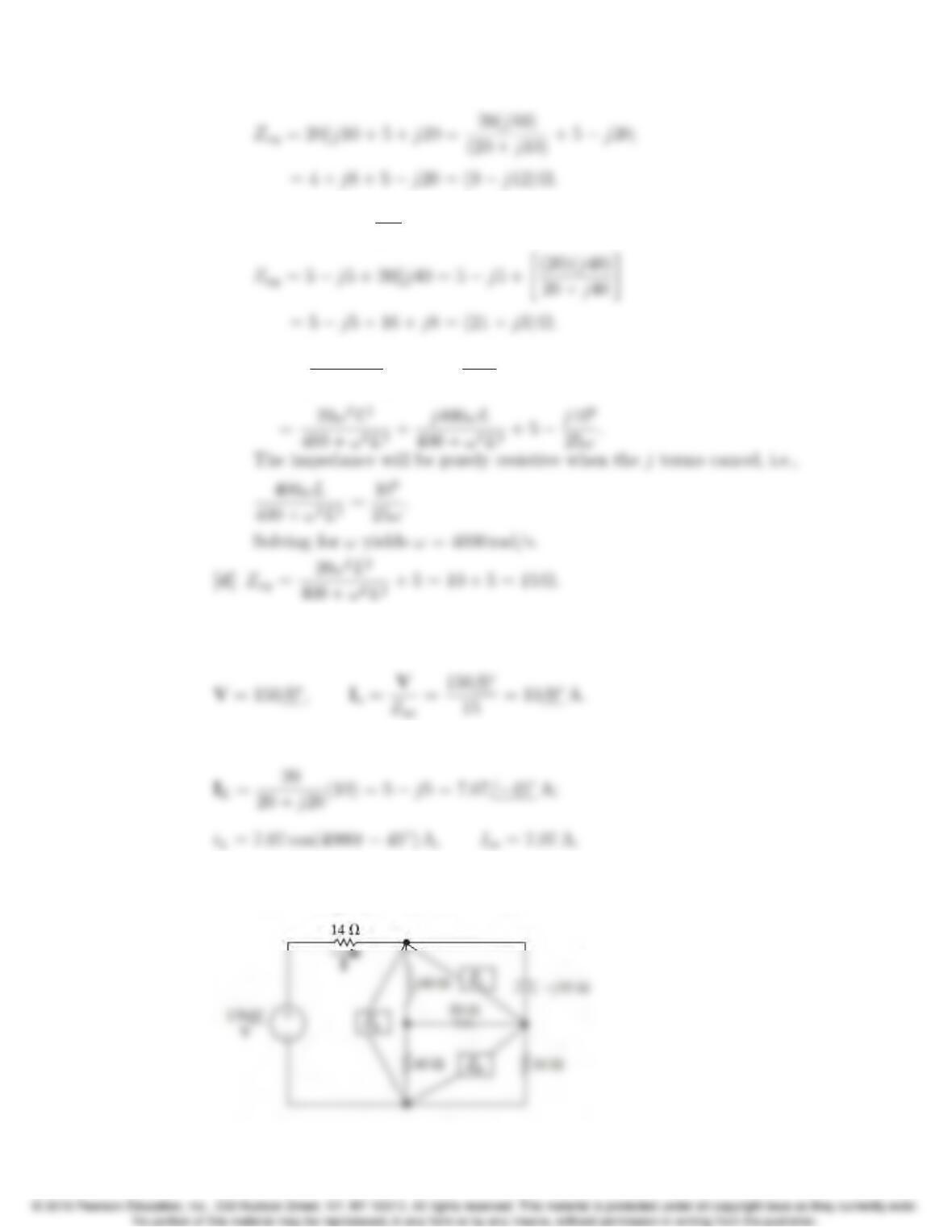
AP 9.7 [a]
Problems 9–3
[b] ωL= 40 Ω,1
ωC=5Ω;
[c] Zxy =“20(jωL)
20 + jωL#+ 5j106
25ω!
AP 9.8 The frequency 4000 rad/s was found to give Zxy = 15 Ωin Assessment
Problem 9.7. Thus,
Using current division,
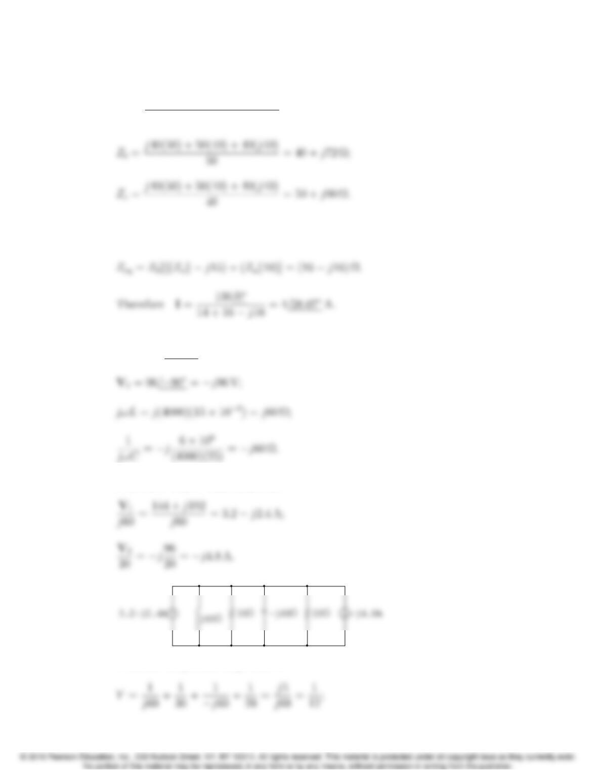
AP 9.9 After replacing the wye made up of the j40 Ω,50 Ω,and 40 Ωimpedances with
its equivalent delta, the circuit becomes
9–4 CHAPTER 9. Sinusoidal Steady State Analysis
where
Za=j40(50) + 50(40) + 40(j40)
j40 = 90 j50 Ω;
The circuit is further simplified by combining the impedances to the right of
the 14 Ωresistor into a single equivalent impedance:
AP 9.10
V1= 240/53.13= 144 + j192 V;
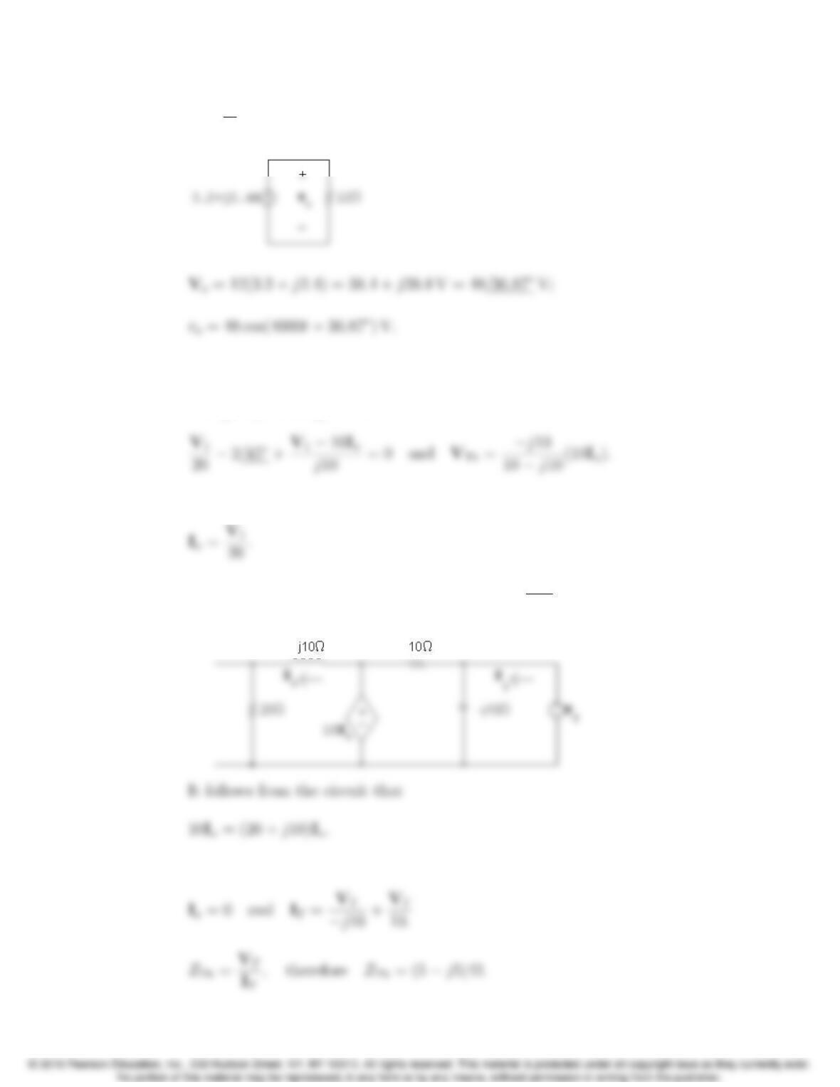
Perform a source transformation:
Combine the parallel impedances:
Problems 9–5
Z=1
Y= 12 Ω.
AP 9.11 Use the lower node as the reference node. Let V1= node voltage across the
20 Ωresistor and VTh = node voltage across the capacitor. Writing the node
voltage equations gives us
We also have
Solving these equations for VTh gives VTh = 10/45V. To find the Th´evenin
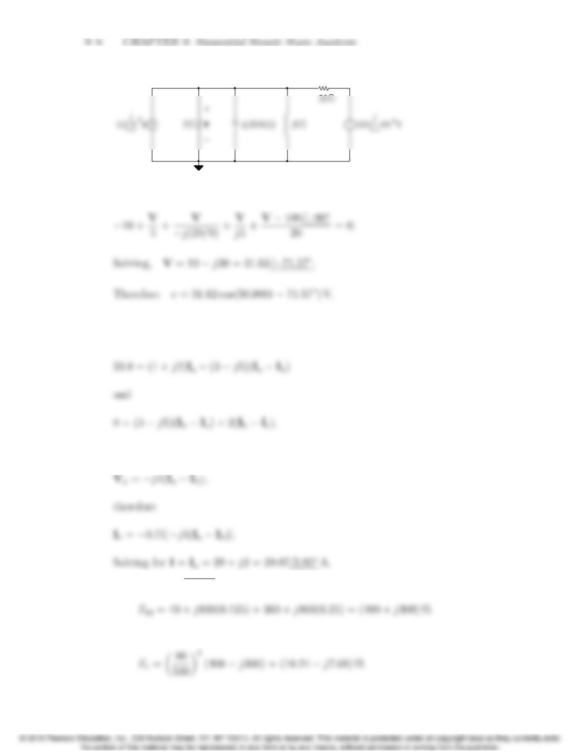
impedance, we remove the independent current source and apply a test
voltage source at the terminals a, b. Thus
Therefore
AP 9.12 The phasor domain circuit is as shown in the following diagram:
The node voltage equation is
AP 9.13 Let Ia,Ib,and Icbe the three clockwise mesh currents going from left to
right. Summing the voltages around meshes a and b gives
But
AP 9.14 [a] M=0.4p0.0625 = 0.1H,ωM= 80 Ω;
Therefore |Z22|= 500 Ω,Z
⇤
22 = (400 j300) Ω.
Problems 9–7
AP 9.15
I1=Vs
Z1+2s2Z2
=25 ⇥103/0
1500 + j6000 + (25)2(4 j14.4)
9–8 CHAPTER 9. Sinusoidal Steady State Analysis
Problems
P 9.1 [a] 40 V.
360(60)=π
3=1.05 rad.
[e] θ= 60.
P 9.2 [a] ω=2πf= 3769.91 rad/s,f=ω
[f] v(t) = 0 when 3769.19t53.13= 90. Now resolve the units:
P 9.3 [a] T
2= 8 + 2 = 10 ms; T= 20 ms;
[b] v=Vmsin(ωt+θ);
P 9.4
P 9.5 [a] By hypothesis
[b] f=ω
2π= 159.155 Hz; T=1
f=6.28 ms;
9–10 CHAPTER 9. Sinusoidal Steady State Analysis
P 9.7 Zto+T
to
V2
mcos2(ωt+φ)dt =V2
mZto+T
to
1
2+1
2cos(2ωt+2φ)dt
P 9.8 Vrms =s1
TZT/2
0V2
msin22π
Tt dt;
P 9.9 [a] From Eq. 9.7 we have
Ldi
dt =VmRcos(φθ)
pR2+ω2L2e(R/L)tωLVmsin(ωt+φθ)
pR2+ω2L2;
But
Problems 9–11
[b] iss =Vm
pR2+ω2L2cos(ωt+φθ).
Therefore
P 9.10 [a] The numerical values of the terms in Eq. 9.6 are
Vm= 20, R/L = 1066.67,ωL= 60;
[b] Transient component = 195.72e1066.67tmA;
P 9.11 [a] Y = 50/60+ 100/30= 111.8/3.43;
[c] Y = 80/30100/225+50
/90= 161.59/29.96;
P 9.12 [a] Vg= 300/78;Ig=6
/33;
[b] iglags vgby 45:
[b] θv=0
;
P 9.14 [a] ω=2πf= 314,159.27 rad/s.
[b] I =V
ZC
=10 ⇥103/0
1/jωC=jωC(10 ⇥103)/0= 10 ⇥103ωC/90;
[d] C=1
15.92(ω)=1
(15.92)(100π⇥103);
P 9.15 [a] ZL=j(8000)(5 ⇥103)=j40 Ω;
Problems 9–13
P 9.16 [a] jωL=j(2 ⇥104)(300 ⇥106)=j6Ω;
[b] Vo= 922/30Ze;
P 9.17 [a] Y=1
3+j4+1
16 j12 +1
j4
9–14 CHAPTER 9. Sinusoidal Steady State Analysis
[d] I =8
/0A,V=I
Y=8
0.2/36.87= 40/36.87V;
P 9.18 [a] Z1=R1+jωL1;
2+ω2L2
2
2+ω2L2
2
P 9.19 [a] Y2=1
R2j
ωL2
;
P 9.20 [a] Z1=R1j1
ωC1
;
Problems 9–15
[b] R1=1000
1 + (40 ⇥103)2(1000)2(50 ⇥104)2= 200 Ω;
P 9.21 [a] Y2=1
R2
+jωC2;
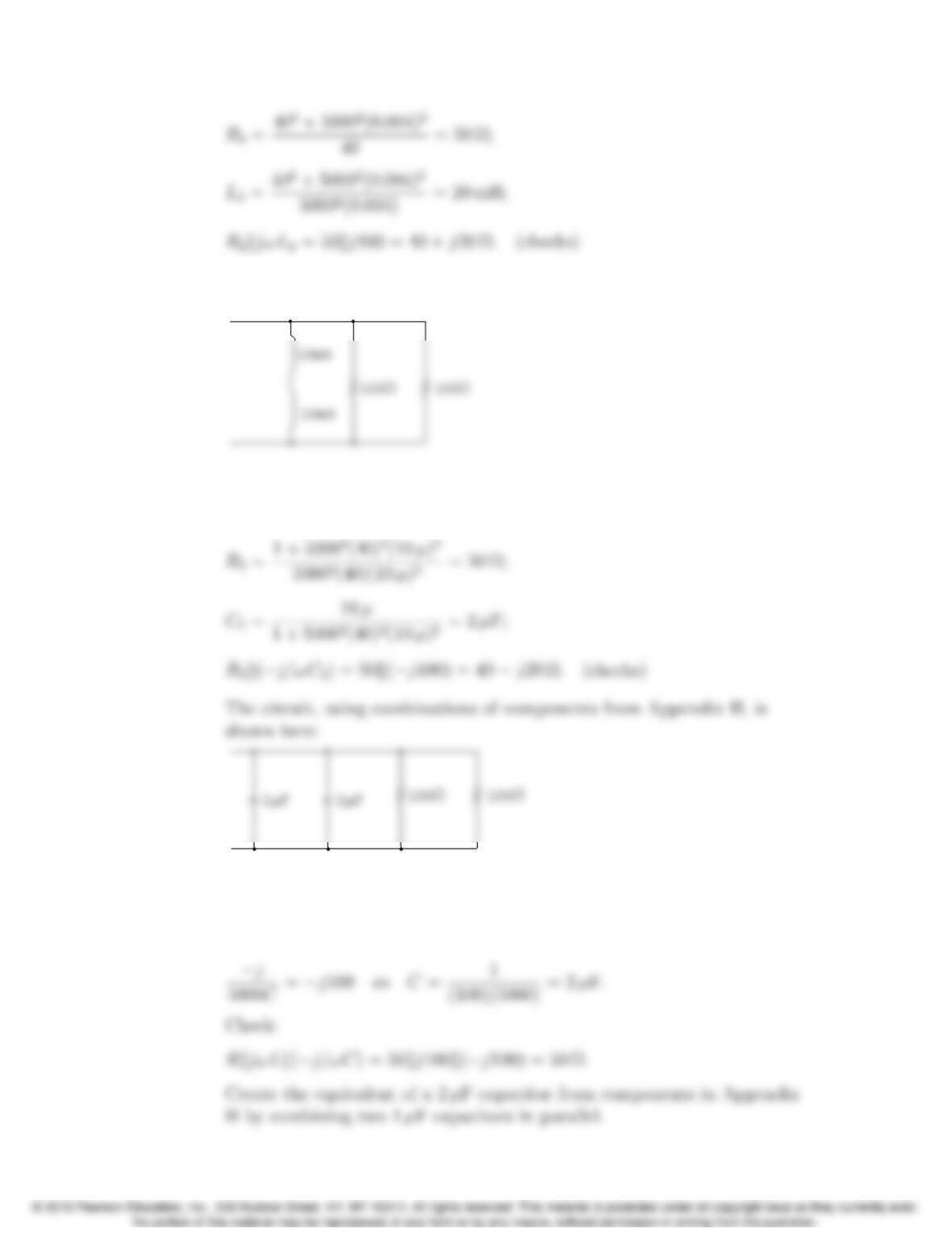
P 9.22 [a] R= 300 Ω= 120 Ω+ 180 Ω;
We can achieve the desired capacitance by combining two 0.1µF
capacitors in parallel. The final circuit is shown here:
P 9.23 [a] Using the notation and results from Problem 9.19:
9–16 CHAPTER 9. Sinusoidal Steady State Analysis
The circuit, using combinations of components from Appendix H, is
shown here:
[b] Using the notation and results from Problem 9.21:
RkC= 40 j20 so R1= 40,C
1= 10 µF;
P 9.24 [a] (40 + j20)k(j/ωC)=50kj100k(j/ωC).
To cancel out the j100 Ωimpedance, the capacitive impedance must be
j100 Ω:
Problems 9–17
[b] (40 j20)k(jωL)=50k(j100)k(jωL).
To cancel out the j100 Ωimpedance, the inductive impedance must be
j100 Ω:
P 9.25 First find the admittance of the parallel branches
Yp=1
6j2+1
4+j12 +1
5+1
j10 =0.375 j0.125 S;
P 9.26 Zab =1j8+(2+j4)k(10 j20) + (40kj20)
P 9.27 [a] jωL=Rk(j/ωC)=jωL+jR/ωC
Rj/ωC
9–18 CHAPTER 9. Sinusoidal Steady State Analysis
·
.. ω
2C2R2+1= CR2
L;
P 9.28 1
jωC=1
(1 ⇥106)(50 ⇥103)=j20 Ω;
P 9.29 Z=4+j(50)(0.24) j1
(50)(0.0025) =5.66/45Ω;
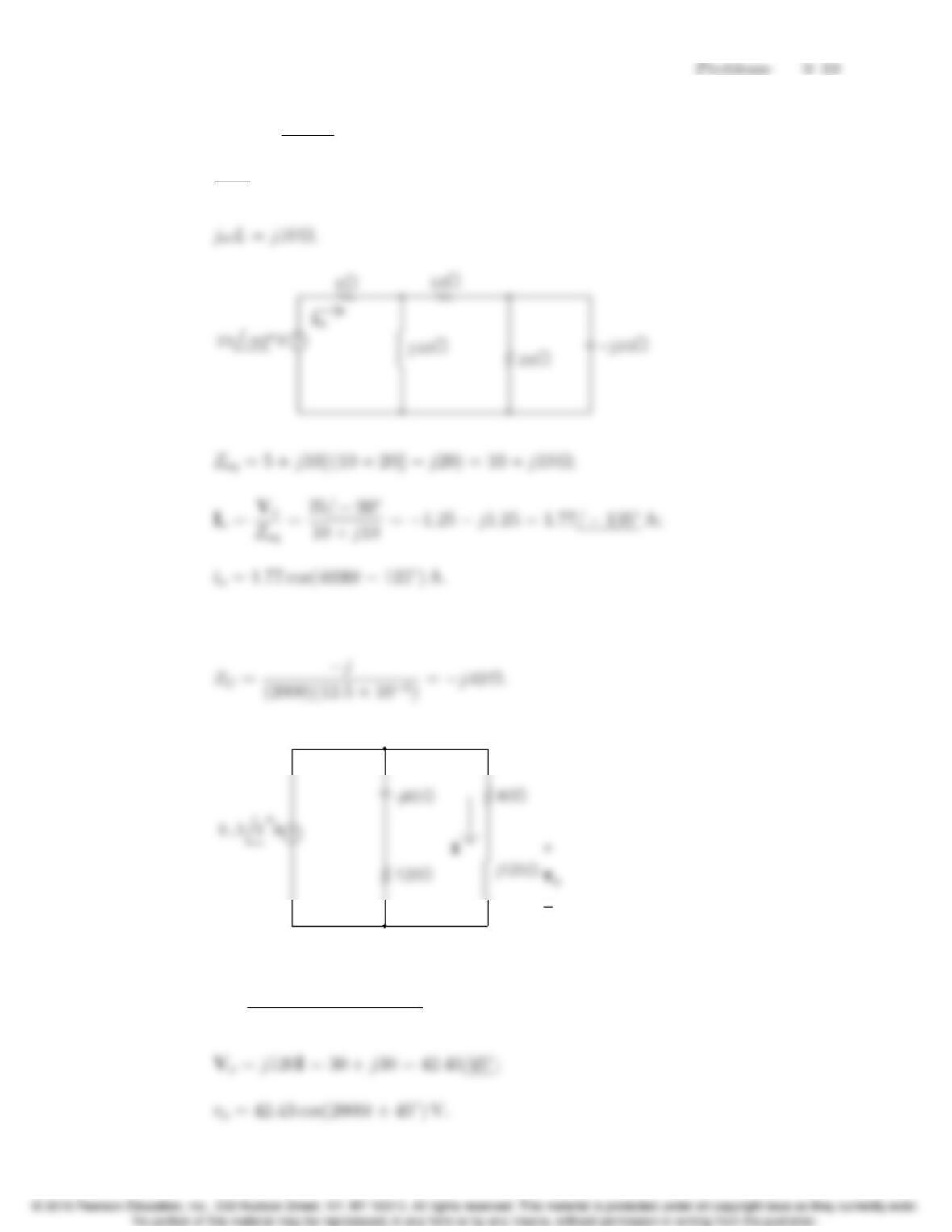
P 9.30 Vs= 25/90V;
1
jωC=j20 Ω;
P 9.31 ZL=j(2000)(60 ⇥103)=j120 Ω;
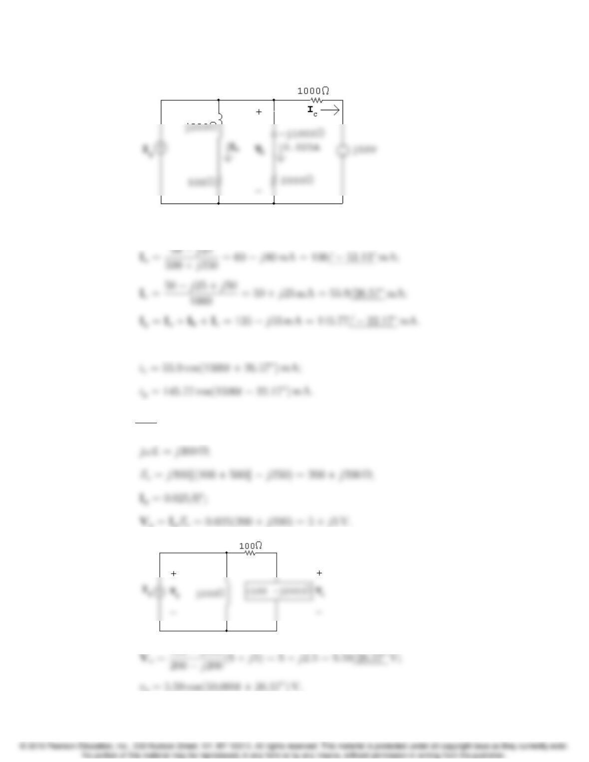
Construct the phasor domain equivalent circuit:
Using current division:
I=(120 j40)
120 j40 + 40 + j120(0.5) = 0.25 j0.25 A;
9–20 CHAPTER 9. Sinusoidal Steady State Analysis
P 9.32 [a]
Vb= (2000 j1000)(0.025) = 50 j25 V;
[b] ia= 100 cos(1500t53.13) mA;
P 9.33 [a] 1
jωC=j250 Ω;