CHAPTER 6
Exercises
E6.1 (a) The frequency of
)20002cos(2)(
in
ttv
is 2000 Hz. For this
E6.2 The input signal
)15002cos(3)205002cos(2)(
tttv
has two
components with frequencies of 500 Hz and 1500 Hz. For the 500-Hz
component we have:
E6.3 The input signal
)30002cos(3)10002cos(21)(
tttv
has three
components with frequencies of 0, 1000 Hz and 3000 Hz.
For the 3000-Hz component:
Thus, the output for all three components is
out
E6.4 Using the voltage-division principle, we have:
R
B
in
E6.5 From Equation 6.9, we have
Hz 200)2/(1
RCfB
, and from Equation
For the first component of the input, the frequency is 20 Hz,
For the second component of the input, the frequency is 500 Hz,
For the third component of the input, the frequency is 10 kHz,
E6.7 (a)
dB 15)(log20)( dB
fHfH
E6.8 (a)
Hz 400021000 2
is two octaves higher than 1000 Hz.
E6.9 (a) To find the frequency halfway between two frequencies on a
E6.10 To determine the number of decades between two frequencies we take
the difference between the common (base-ten) logarithms of the two
Similarly, to determine the number of octaves between two frequencies
E6.11 The transfer function for the circuit shown in Figure 6.17 in the book is
E6.12 Using the voltage division principle, the transfer function for the circuit
shown in Figure 6.19 in the book is
E6.13 Using the voltage division principle, the transfer function for the circuit
shown in Figure 6.22 in the book is
E6.14 A first-order filter has a transfer characteristic that decreases by 20
dB/decade below the break frequency. To attain an attenuation of 50 dB
E6.15
pF 2533
1010)102(
1
)2(
11
6262
0
2
0
LfL
C
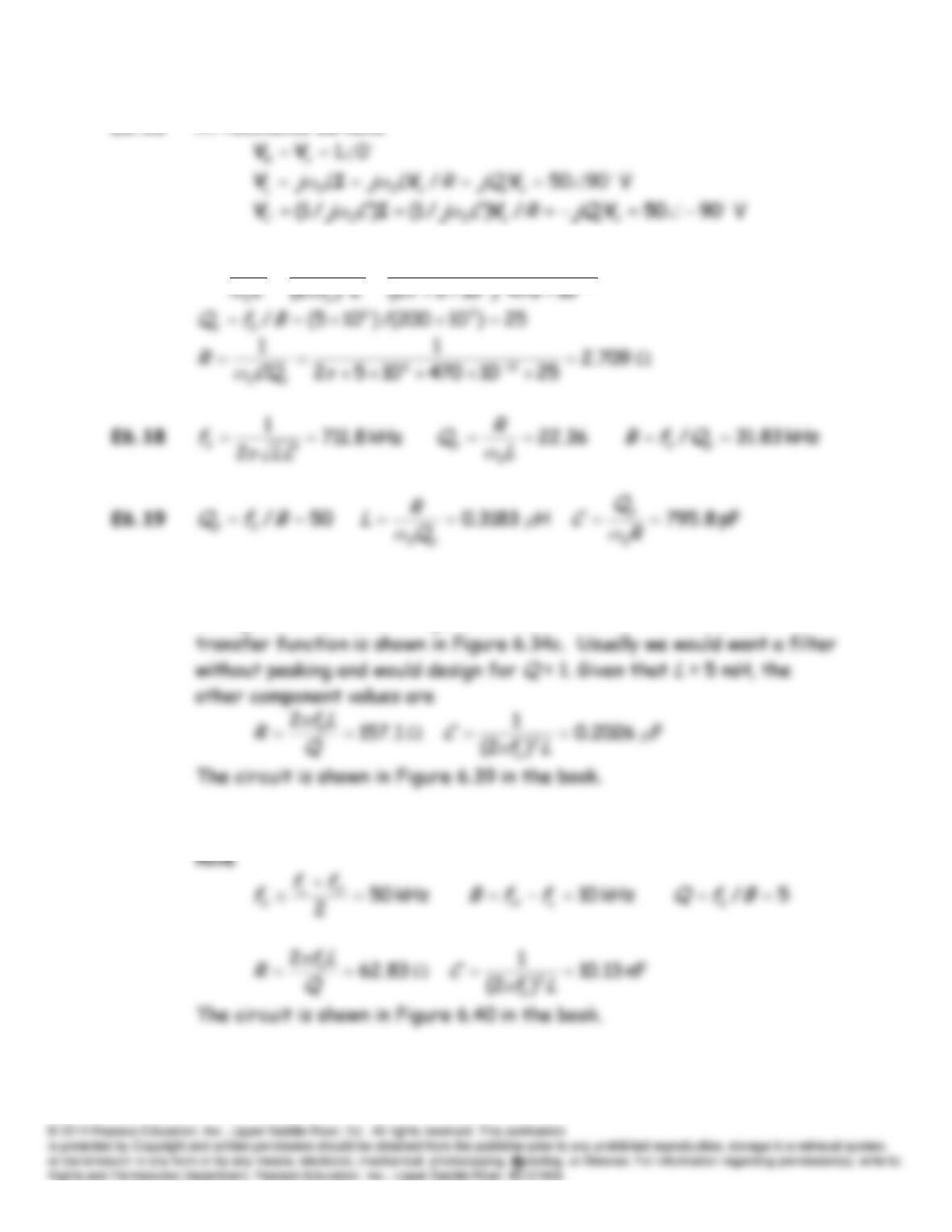
E6.16 At resonance we have
E6.17
H 156.2
1
11
12262
2
L
E6.20 A second order lowpass filter with
f
0 = 5 kHz
is needed. The circuit
configuration is shown in Figure 6.34a in the book. The normalized
E6.21 We need a bandpass filter with
kHz. 55 and kHz 45
HL ff
Thus we
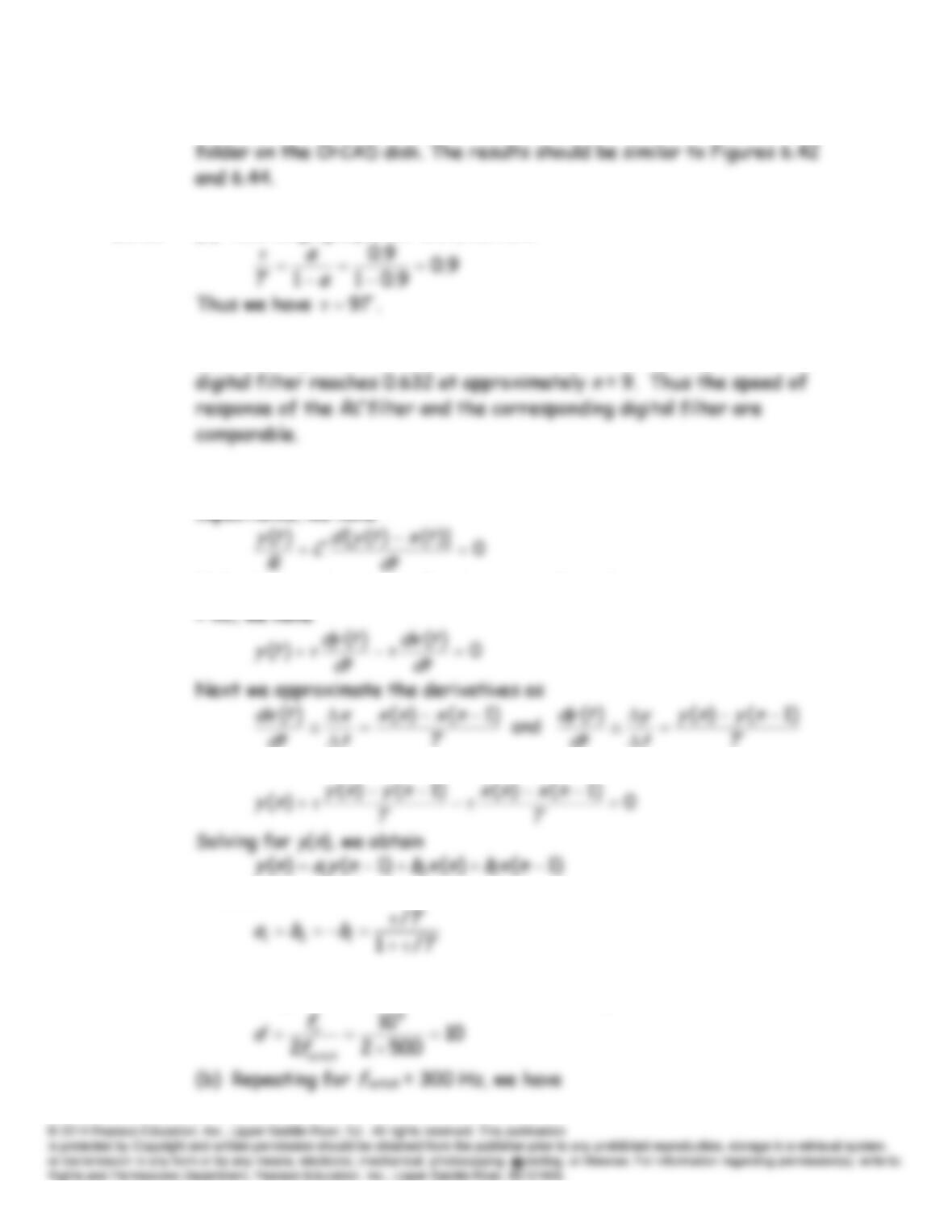
E6.22 The files Example_6_8 and Example_6_9 can be found in the MATLAB
E6.23 (a) Rearranging Equation 6.56, we have
(b) From Figure 6.49 in the book we see that the step response of the
E6.24 Writing a current equation at the node joining the resistance and
capacitance, we have
Multiplying both sides by
R
and using the fact that the time constant is
which yields
in which
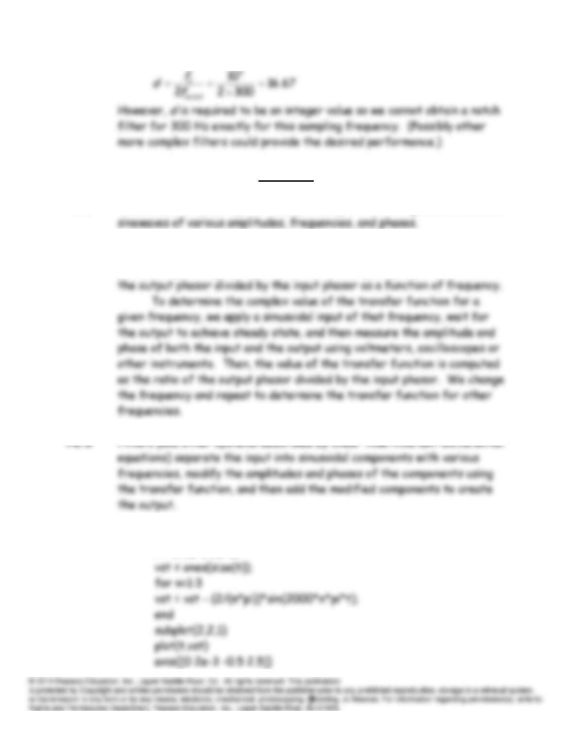
E6.25 (a) Solving Equation 6.58 for
d
and substituting values, we obtain
Problems
P6.1 The fundamental concept of Fourier theory is that all signals are sums of
P6.2 The transfer function shows how a filter affects the amplitude and
phase of input components as a function of frequency. It is defined as
P6.4 A MATLAB program to create the plots is:
t = 0:2e-6:2e-3;
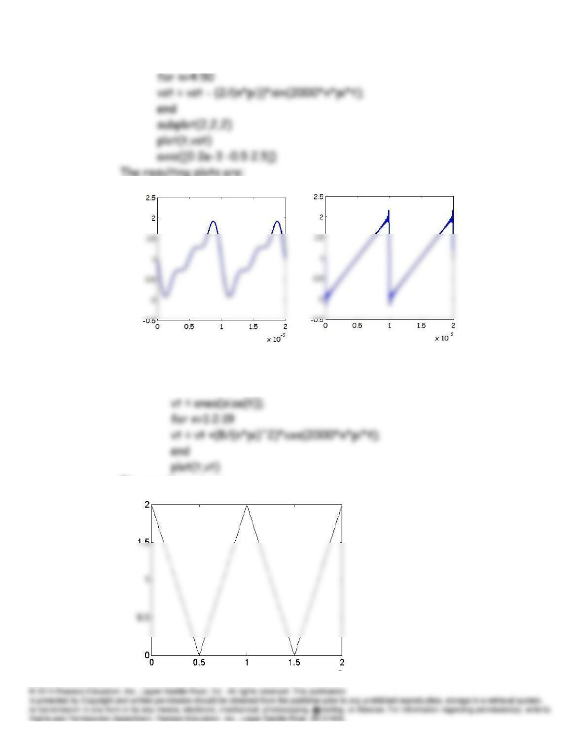
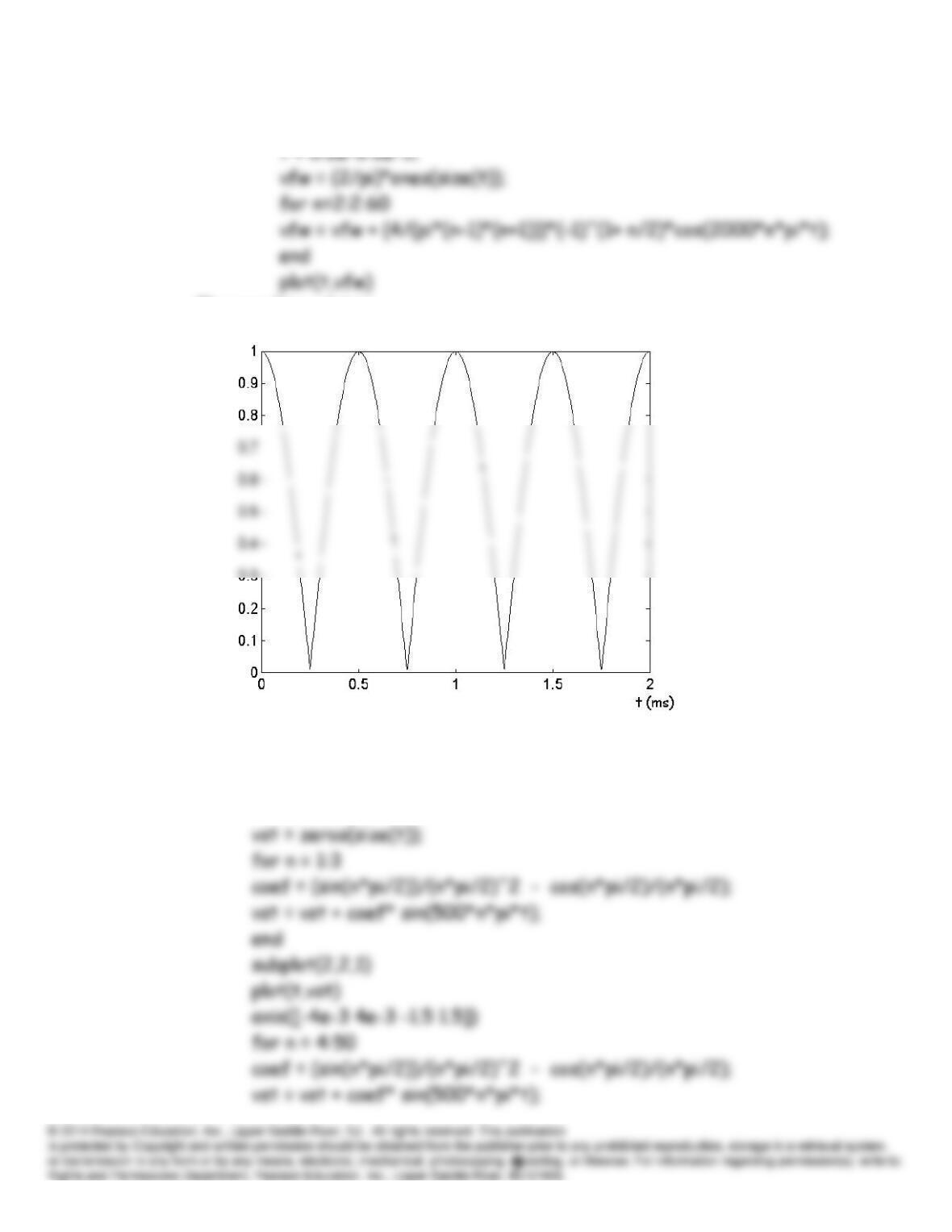
P6.5 A MATLAB program to create the plot is:
t = 0:2e-6:2e-3;
The resulting plot is:
t
(ms)
P6.6 A MATLAB program to create the plot is:
The resulting plot is:
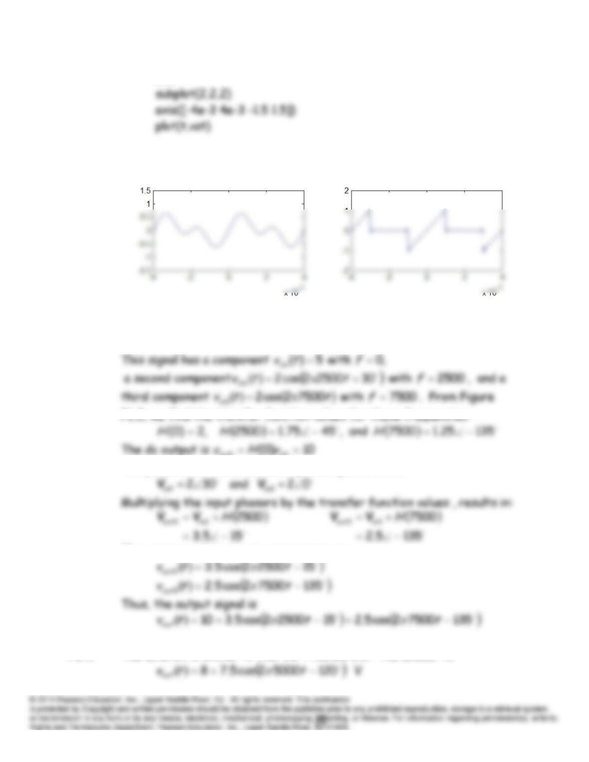
P6.7 A MATLAB program to create the plots is:
clear
t = -4e-3:2e-6:4e-3;
end
The resulting plots are:
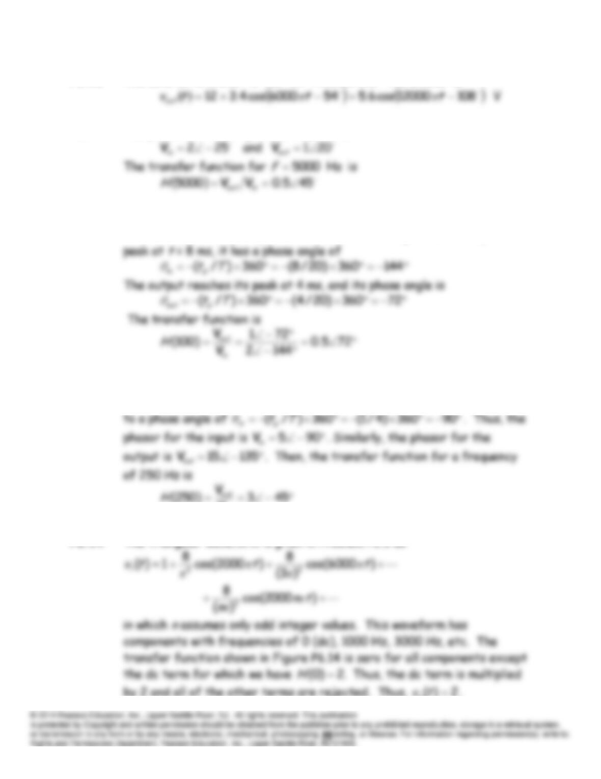
P6.8* The given input signal is
tttvin
75002cos23025002cos25
inout vHv
The phasors for the sinusoidal input components are
The corresponding output components are:
P6.9 The solution is similar to that for Problem 6.8. The answer is:
P6.10 The solution is similar to that for Problem 6.8. The answer is:
P6.11* The phasors for the input and output are:
P6.12 From Figure P6.12, we see that the period of the signals is 20 ms.
Therefore, the frequency is 50 Hz. Because the input reaches a positive
P6.13* The input has a peak value of 5 V and reaches a positive peak at 1 ms.
Since the period is 4 ms, the frequency is 250 Hz and 1 ms corresponds
in
V
P6.14* The triangular waveform is given in Problem P6.5 as
by 2 and all of the other terms are rejected. Thus,
2)(
tvo
.
P6.15* Given
in
ftVtv
max
2cos
π
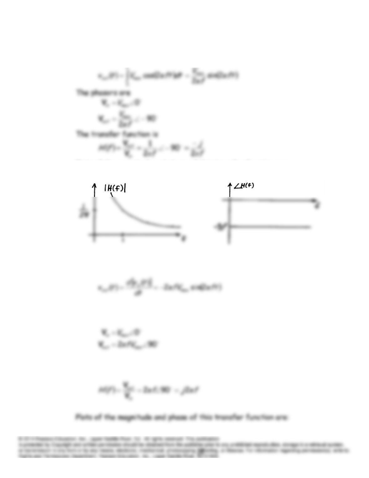
Plots of the magnitude and phase of this transfer function are:
P6.16 Given
ftVtvin
π2cos max
The phasors are
The transfer function is
P6.17 The input signal given in Problem P6.4 is:
The frequencies of the various components are
f
0, 1000, 2000, 3000,
P6.18
ftVtvin
π2cos
max
The phasors are
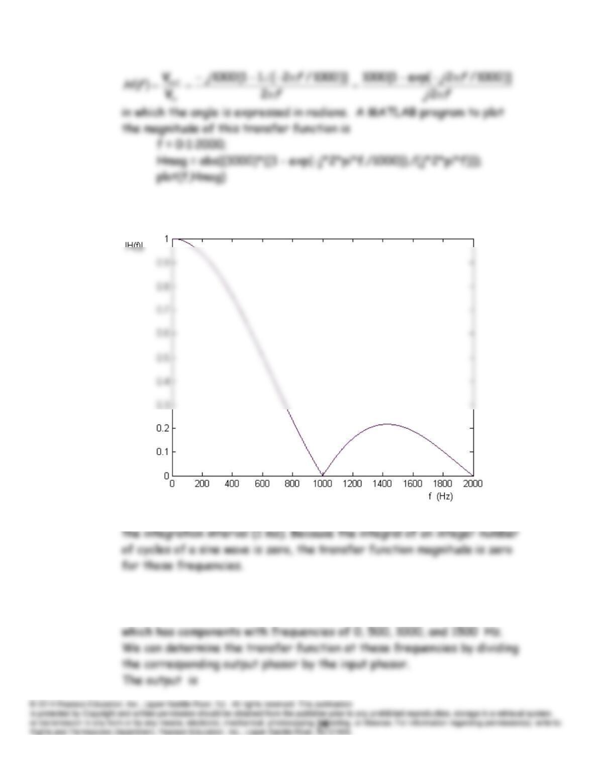
The resulting plot of the magnitude of the transfer function is:
For integer multiples of 1000 Hz, an integer multiple of cycles appear in
P6.19 The input signal is
ttttv
3000cos2000sin31000cos32
in
P6.20
ftVtvin
π2cos
max
)]102(2cos[2cos 3
maxmax
tfVftVtvout
in
in which the angle is expressed in radians.
A MATLAB program to plot the magnitude of this transfer function is
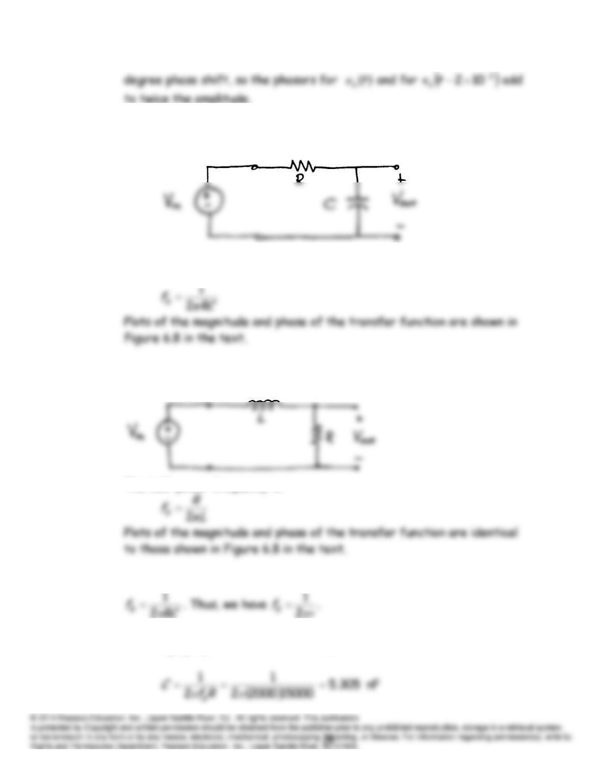
A plot of the magnitude of the transfer function is:
For a 250 Hz sinewave, a delay of 2 ms corresponds to a 180 degree
P6.21 The circuit diagram is:
The half-power frequency is:
P6.22 The circuit diagram of a first-order
RL
lowpass filter is:
The half-power frequency is:
P6.23 The time constant is given by
RC
and the half-power frequency is
P6.24 Rearranging Equation 6.8 in the text yields:
P6.25* The phase of the transfer function is given by Equation 6.11 in the text:
B
fffH
arctan
P6.26* The half-power frequency of the filter is
Hz 500
2
1
RC
fB
π
The transfer function is given by Equation 6.9 in the text:
B
ffj
fH
1
1
P6.27 The transfer function is given by Equation 6.9 in the text:
B
ffj
fH
1
1
The given input signal is
P6.28 The period of a 5-kHz sinusoid is 200 s. The phase shift corresponding
to a delay of 20 s is
36
. (We give the phase shift as negative
B
P6.29 To achieve a reduction of the 20-kHz component by a factor of 100, we
must have
P6.30* The circuit seen by the capacitance is:
The open-circuit or Thévenin voltage is
Zeroing the source, we have
Thus, the equivalent circuit is:
As in the text, this circuit has the transfer function:
t
Using Equation (1) to substitute for
t
V
in Equation (2) and rearranging, we
P6.31 The input and output voltages given have a frequency of 10 kHz. Dividing
the output phasor by the input phasor, we obtain the transfer function:
10.0
5.0
)10(
out
4
V
H
P6.32 For the 10-kHz signal, the transfer function magnitude is
1
1
04.0
22.0
)(
out
fH
V
V
P6.33 (a) First, we find the Thévenin equivalent for the source and resistances.