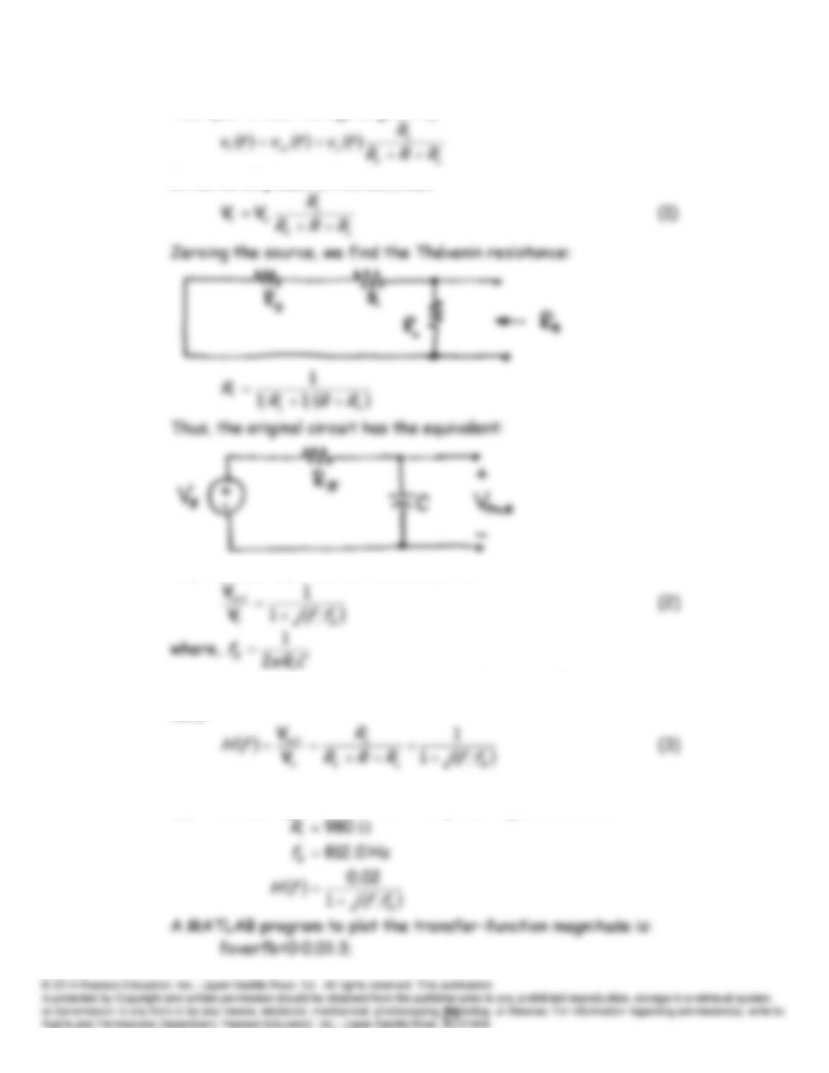
The open-circuit voltage is given by
In terms of phasors, this becomes:
The transfer function for this circuit is:
Using Equation (1) to substitute for
t
V
in Equation (2) and rearranging, we
have:
(b) Evaluating for the circuit components given, we have:
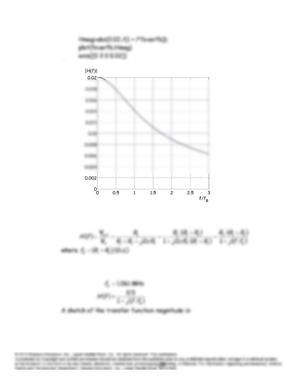
The resulting plot is:
P6.34 (a) Applying the voltage-division principle, we have:
(b) Evaluating for the component values given, we have:
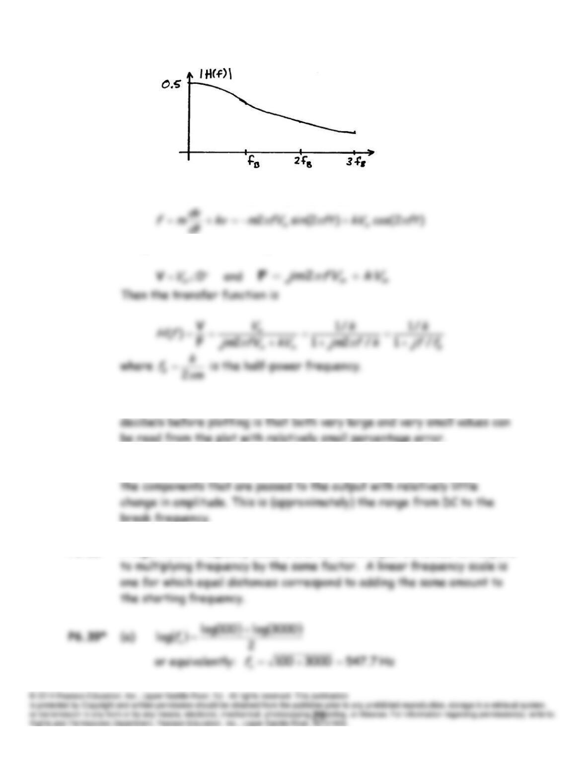
P6.35 With an assumed velocity
)2cos(
ftVv m
, the force is
The phasors for the velocity and the force are
P6.36 The primary advantage of converting transfer-function magnitudes to
P6.37 The passband of a simple
RC
lowpass filter is the range of frequencies of
P6.38 A logarithmic frequency scale is one for which equal distances correspond
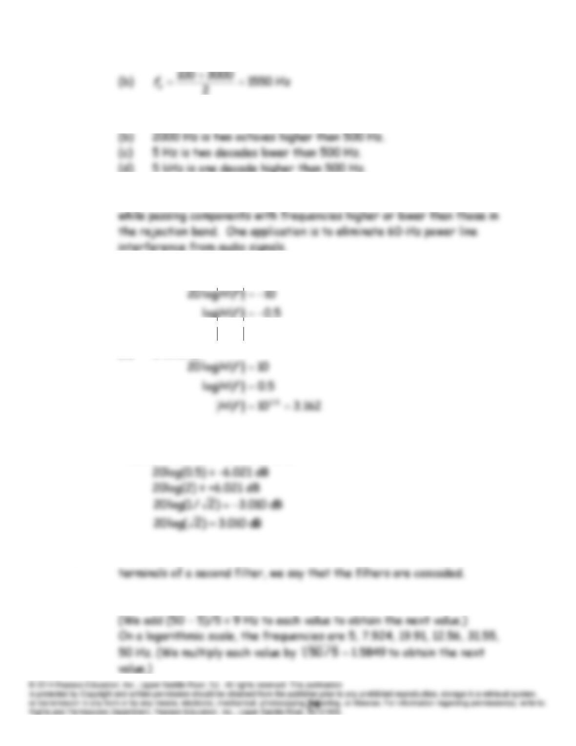
P6.40 (a) 250 Hz is one octave lower than 500 Hz.
P6.41 A notch filter rejects components with frequencies in a narrow band
P6.42* (a) We have:
3162.010
5.0
fH
(b) Similarly,
P6.43 To convert to decibels, we take 20 times the common logarithm of the
transfer function. Thus, we have:
P6.44 If the output terminals of one filter are connected to the input
P6.45 On a linear scale, the frequencies are 5, 14, 23, 32, 41, 50 Hz.
P6.46 (a) We have
100002510
d
N
.
Taking the common logarithm of both sides, we have:
oct
P6.48* (a) The overall transfer function is the product of the transfer
functions of the filters in cascade:
P6.49 For filters in cascade, the transfer functions in decibels are added.
P6.51 The slope of the high-frequency asymptote is -20 dB/decade. The slope
B
P6.52 Because the transfer functions in decibels add for cascaded systems, the
slope declines at 80 dB/decade.
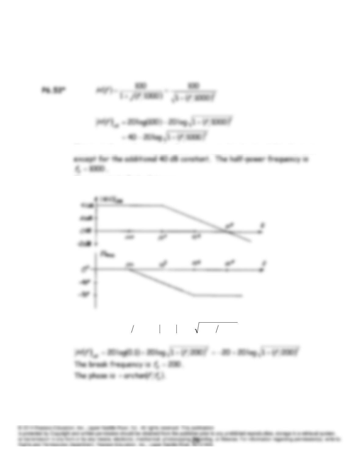
This is similar to the transfer function treated in Section 6.4 in the text
The asymptotic Bode plots are:
P6.54
]2001[1.0
fjfH
2
20011.0
ffH
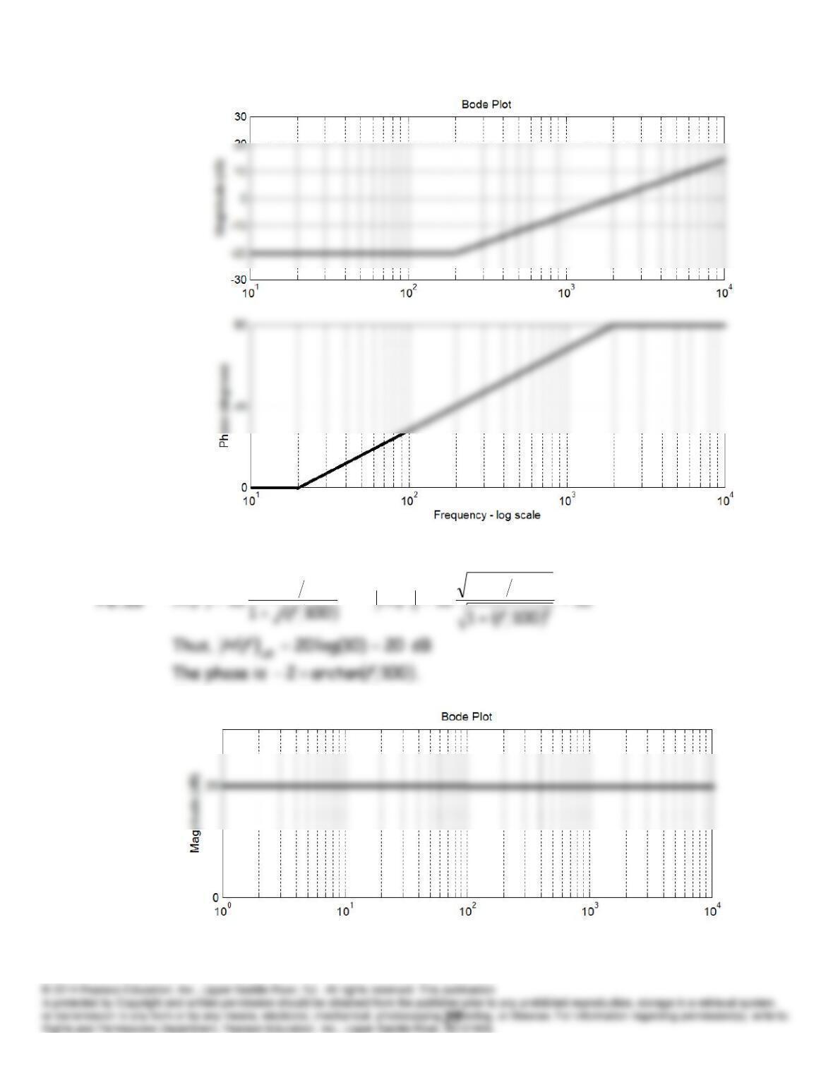
The asymptotic Bode Plots are:
1001
1001
2
f
fj
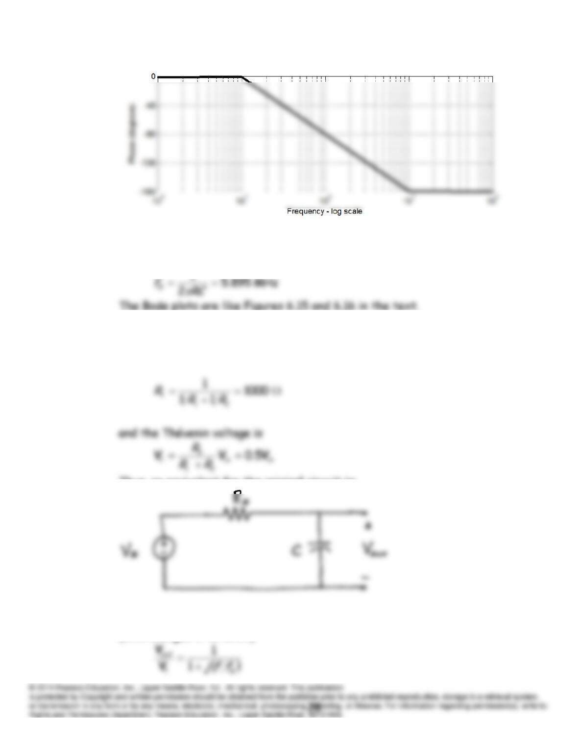
The asymptotic plots are:
P6.56 This is a first-order lowpass
RC
filter. The break frequency is:
P6.57 First, we find the Thévenin equivalent for the source and the resistances.
The Thévenin resistance is
Thus, an equivalent for the original circuit is:
This is a lowpass filter having a transfer function given by Equation 6.8
(with changes in notation):
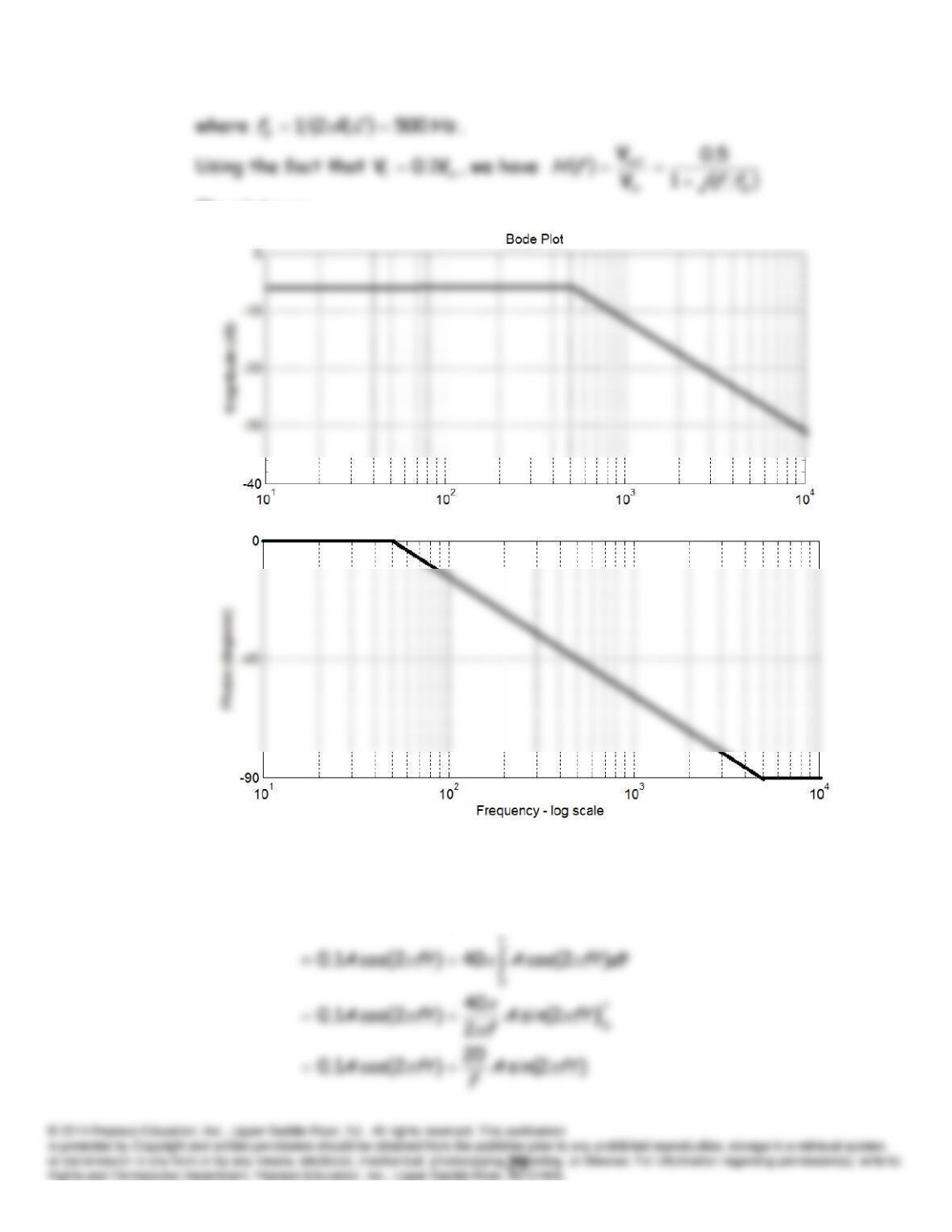
The plots are:
P6.58 (a) Solving for the input voltage, we have
)(40)(1.0)(
0
outout
in
dttvtvtv
t
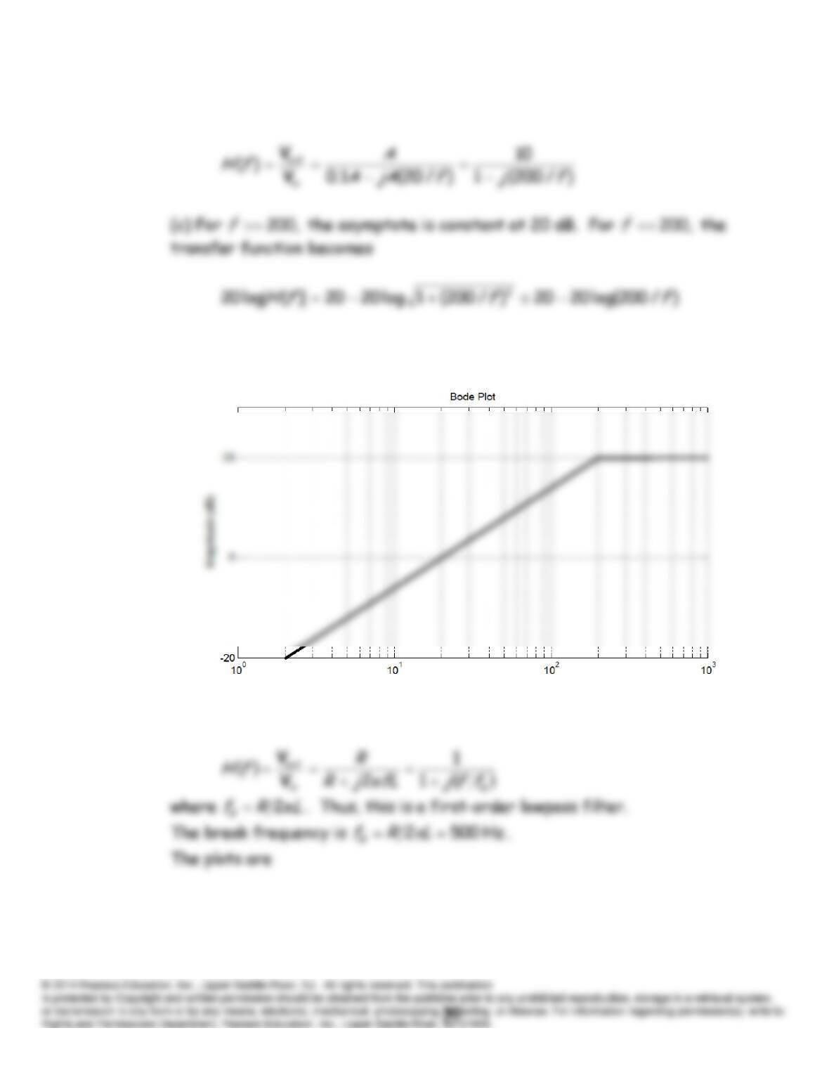
(b) Then the transfer function for the system is
which describes an asymptote sloping downward at 20 dB/decade as
f
becomes smaller. The asymptotic plot for the magnitude is
P6.59 Applying the voltage-division principle, we find the transfer function:
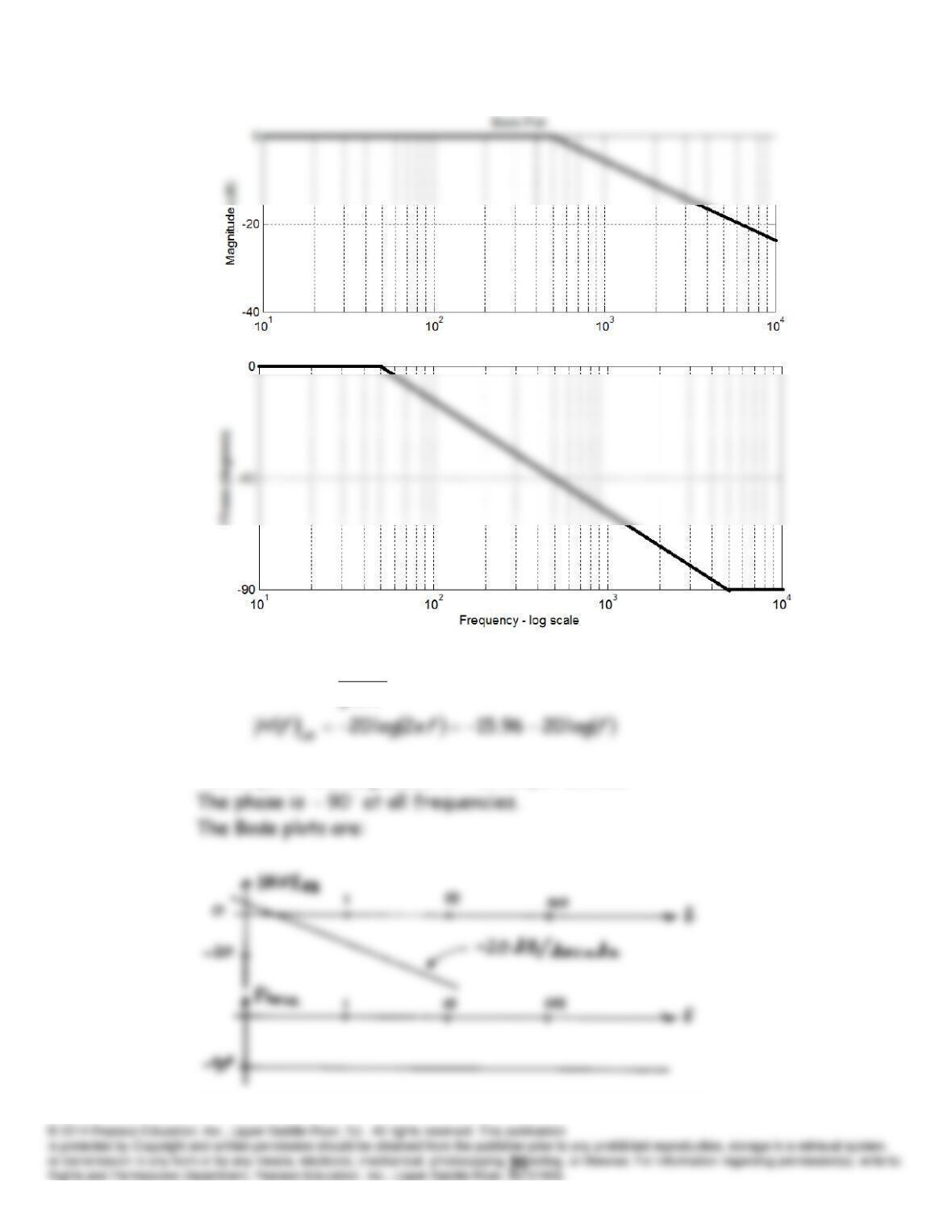
P6.60*
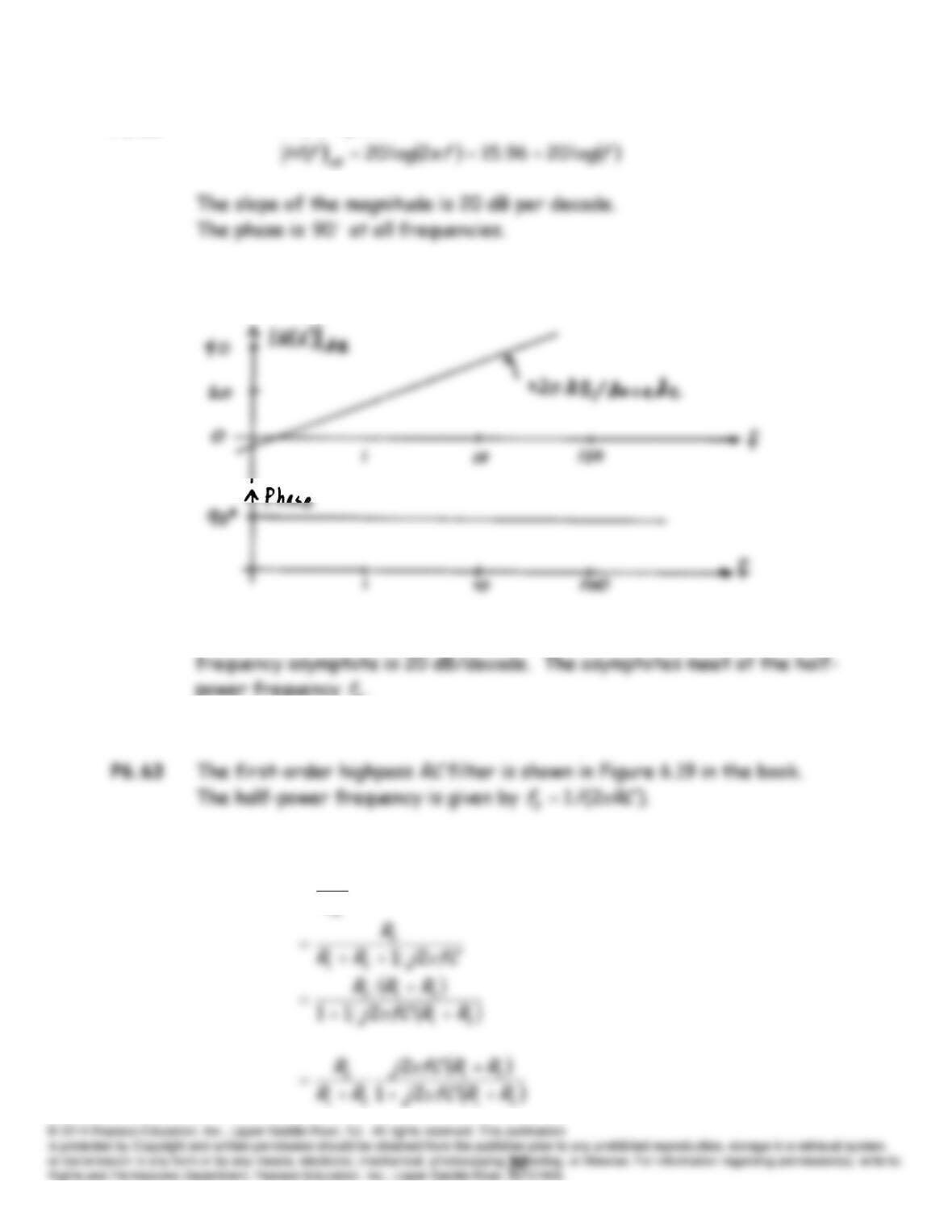
The slope of the magnitude is
20
dB per decade.
fj
fH
2
1
π
P6.61
The Bode plots are:
P6.62 The slope of the high-frequency asymptote is zero. The slope of the low-
B
P6.64* Applying the voltage-division principle, we have:
out
fH
V
V
fjfH
2
π
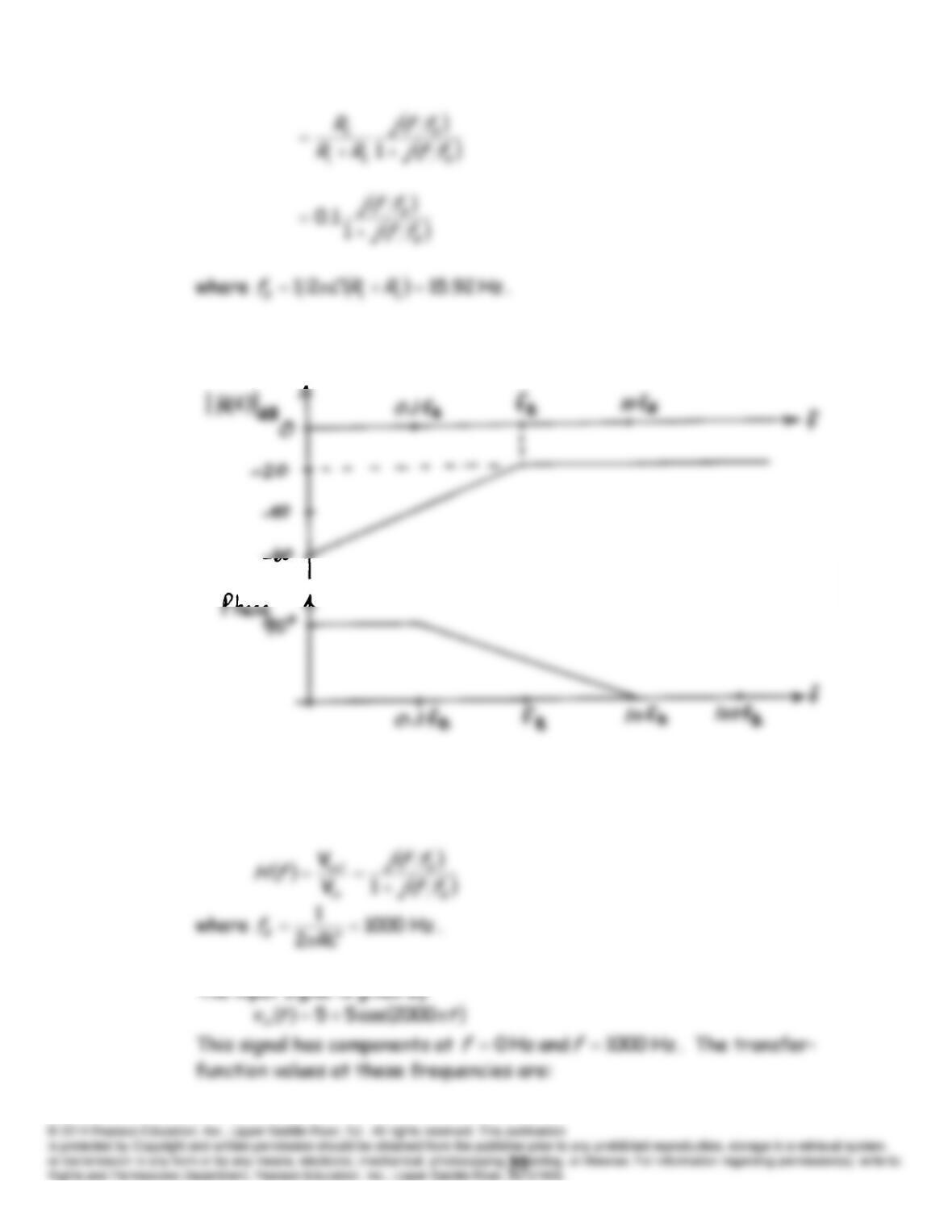
The asymptotic Bode plots are:
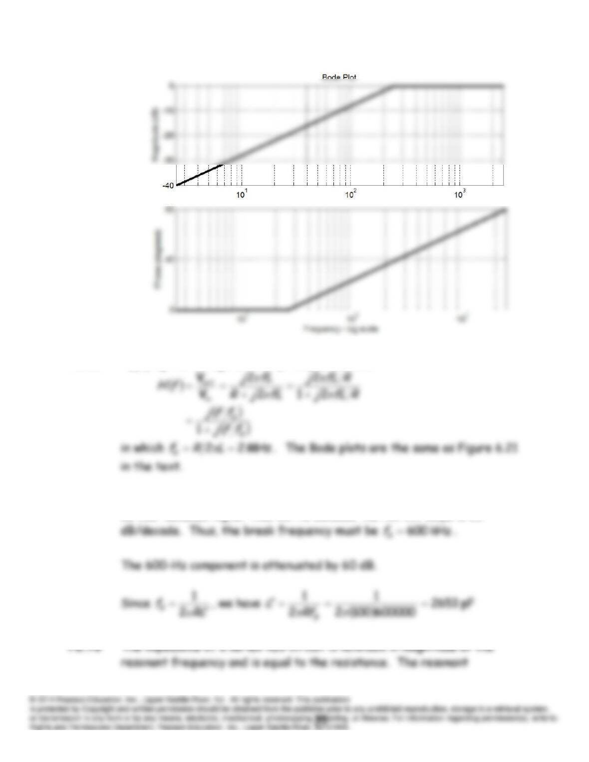
P6.65* This is the first-order high-pass filter analyzed in Section 6.5 in the
text. The transfer function is
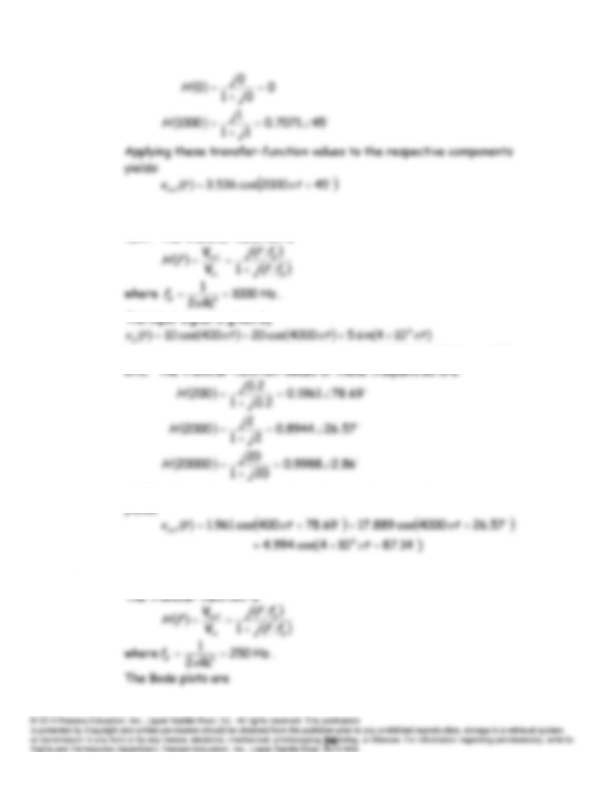
P6.66 This is the first-order high-pass filter analyzed in Section 6.5 in the
text. The transfer function is
This signal has components with frequencies of 200 Hz, 2 kHz and 20
Applying these transfer-function values to the respective components
P6.67 This is a first-order high-pass filter analyzed in Section 6.5 in the text.
P6.68 Applying the voltage-division principle, we have:
P6.69 To attenuate the 60-Hz component by 80 dB, the break frequency must
be four decades higher than 60 Hz because the roll-off slope is 20
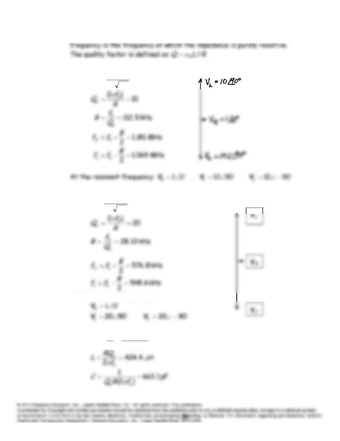
P6.71*
P6.72
At the resonant frequency:
P6.73
20
kHz 15
kHz 300
0
B
f
Qs
MHz 125.1
2
1
0
LC
f
π
kHz 7.562
2
1
0
LC
f
P6.74 The impedance of the circuit is given by
At the resonant frequency, the imaginary part equals zero.
P6.75* Assuming zero phase for
R
V
, the phasor diagram at the resonant
frequency is shown.
and
P6.76
5
min
RZ s
30
MHz 12
0
f
Qs
P6.77 A bandpass filter is a filter that passes components in a band of
frequencies, rejecting components with higher and lower frequencies.
P6.78 The impedance of a parallel
RLC
circuit is maximum in magnitude at the
resonant frequency and is equal to the resistance. The resonant
1
P6.80
k 5
RZ p
P6.81
25
0
B
f
Qp
H 66.63
20
n
Qf
R
L
P6.82
16
0
f
Qp
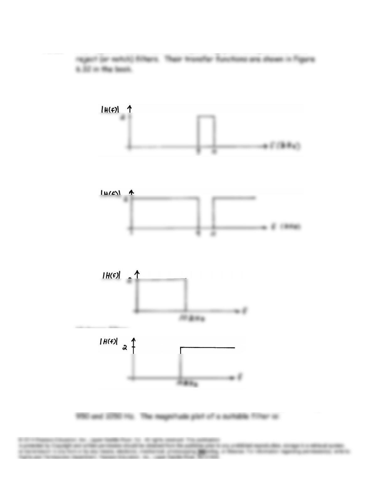
P6.83 Four types of ideal filters are lowpass, highpass, bandpass, and band
P6.84* Bandpass filter:
Band-reject filter:
P6.85 Lowpass filter:
Highpass filter:
P6.86 A band-reject filter is needed with cutoff frequencies of approximately
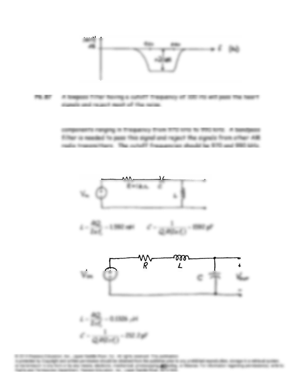
P6.88 An AM radio signal having a carrier frequency of 980 kHz has
P6.89* The circuit diagram of a second-order highpass filter is:
P6.90 The circuit diagram of a second-order lowpass filter is: