Problems 5–19
P 5.29 [a] Assume vais acting alone. Replacing vbwith a short circuit yields vp= 0,
therefore vn= 0 and we have
Therefore
Assume vbis acting alone. Replace vawith a short circuit. Now
vp=vn=vbRd
Rc+Rd
;
[b] Rd
Ra✓Ra+Rb
Rc+Rd◆=Rb
Ra
,therefore Rd(Ra+Rb)=Rb(Rc+Rd);
P 5.30 vp=Rbib=vn;
5–20 CHAPTER 5. The Operational Amplifier
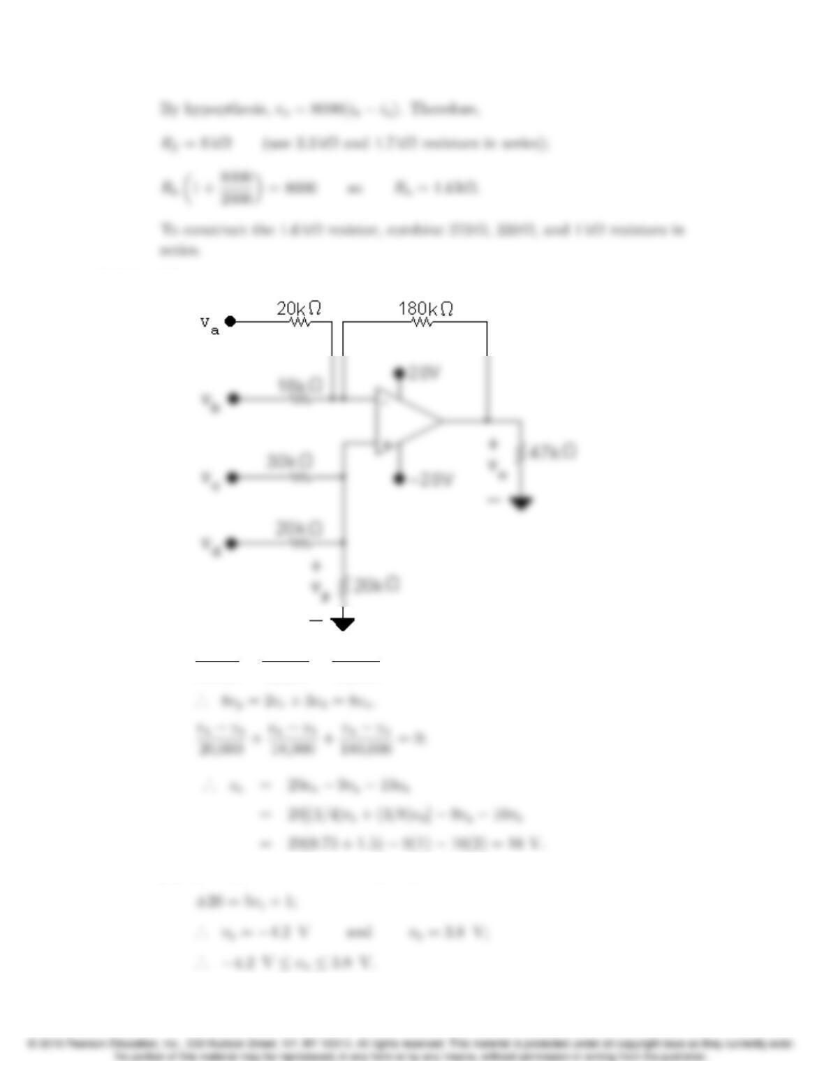
P 5.31 [a]
vp
20,000 +vpvc
30,000 +vpvd
20,000 = 0;
[b] vo=5vc+30920 = 5vc+1;
Problems 5–21
P 5.32 [a] Adm =95(100 + 5) + 100(5 + 95)
2(5)(5 + 95) = 19.975.
P 5.33 Acm =(20)(50) (50)Rx
20(50 + Rx);
P 5.34 [a] vp=αRg
αRg+(RgαRg)vgvo=✓1+Rf
R1◆αvgRf
R1
vg;
αvoαvoαvo
0.08V 0.44V 0.80V
5–22 CHAPTER 5. The Operational Amplifier
[b] Rearranging the equation for vofrom (a) gives
[c] Using the equations from (b),
◆vg;4=✓Rf
P 5.35 [a] vp=vs,v
n=R1vo
R1+R2
,v
n=vp.
P 5.36 It follows directly from the circuit that vo=16vg.
From the plot of vgwe have vg=0,t<0.
vg=t0t0.5;
Problems 5–23
Therefore
vo=16t0t0.5;
These expressions for voare valid as long as the op amp is not saturated.
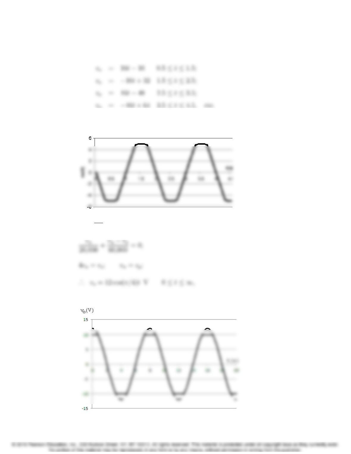
Since the peak values of voare ±5, the output is clipped at ±5. The plot is
shown below.
P 5.37 vp=5.4
7.2vg=0.75vg= 3 cos(π/4)tV;
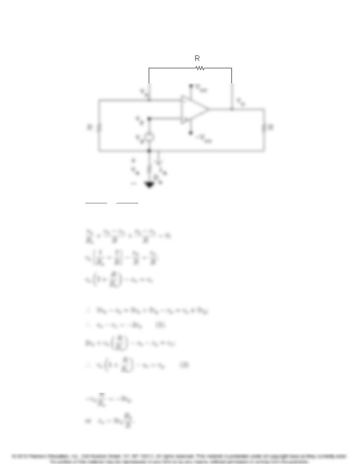
but saturation occurs at vo=±10 V.
5–24 CHAPTER 5. The Operational Amplifier
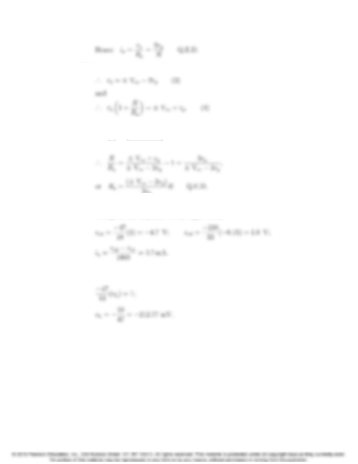
P 5.38 [a]
vnva
R+vnvo
R= 0;
2vnva=vo;
vn=vp=va+vg;
Now combining equations (1) and (2) yields
Problems 5–25
[b] At saturation vo=±Vcc,
Dividing Eq (4) by Eq (3) gives
1+ R
Ra
=±Vcc +vg
±Vcc 2vg
;
3vg
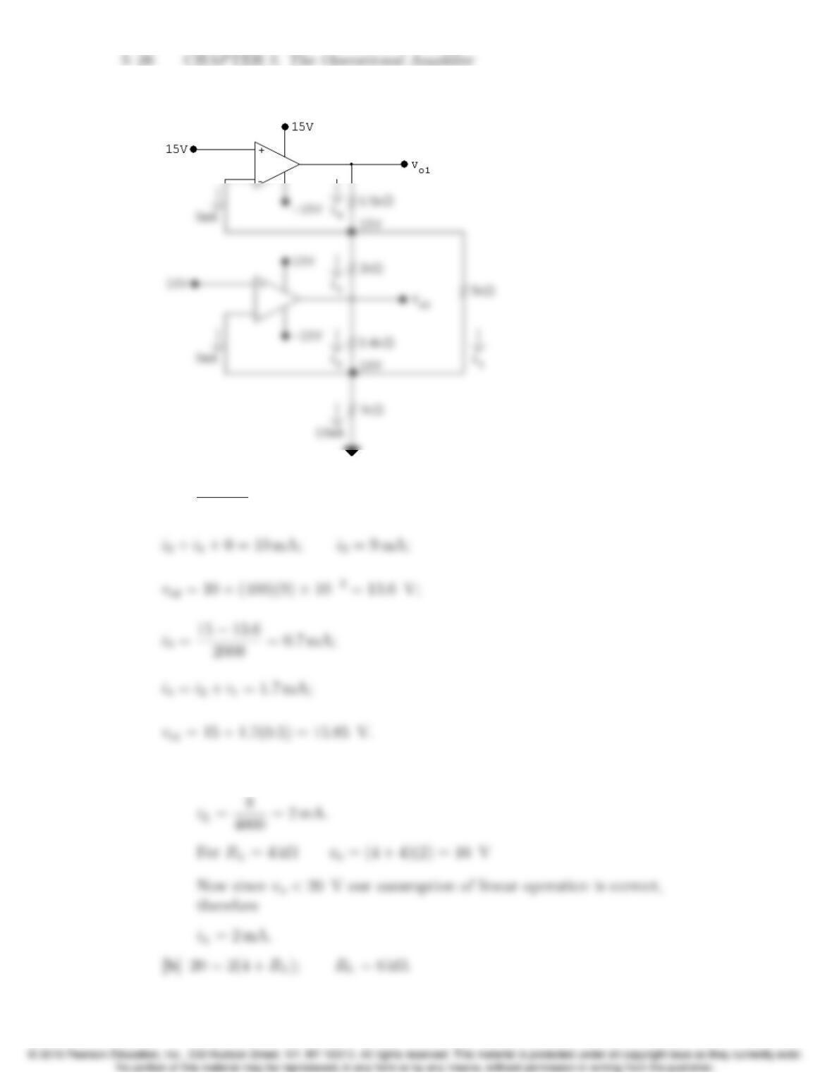
P 5.39 [a] Let vo1= output voltage of the amplifier on the left. Let vo2= output
voltage of the amplifier on the right. Then
[b] ia= 0 when vo1=vo2so from (a) vo2=1 V.
Thus
P 5.40
i1=15 10
5000 = 1 mA;
P 5.41 [a] Assume the op-amp is operating within its linear range, then
Problems 5–27
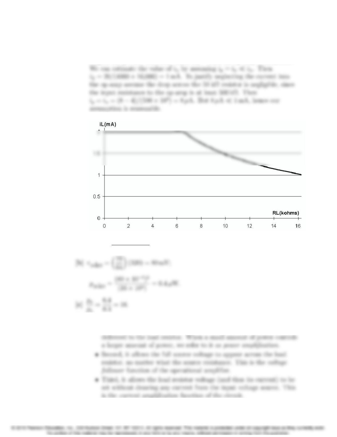
[c] As long as the op-amp is operating in its linear region iLis independent of
RL. From (b) we found the op-amp is operating in its linear region as
long as RL6 kΩ. Therefore when RL= 6 kΩthe op-amp is saturated.
[d]
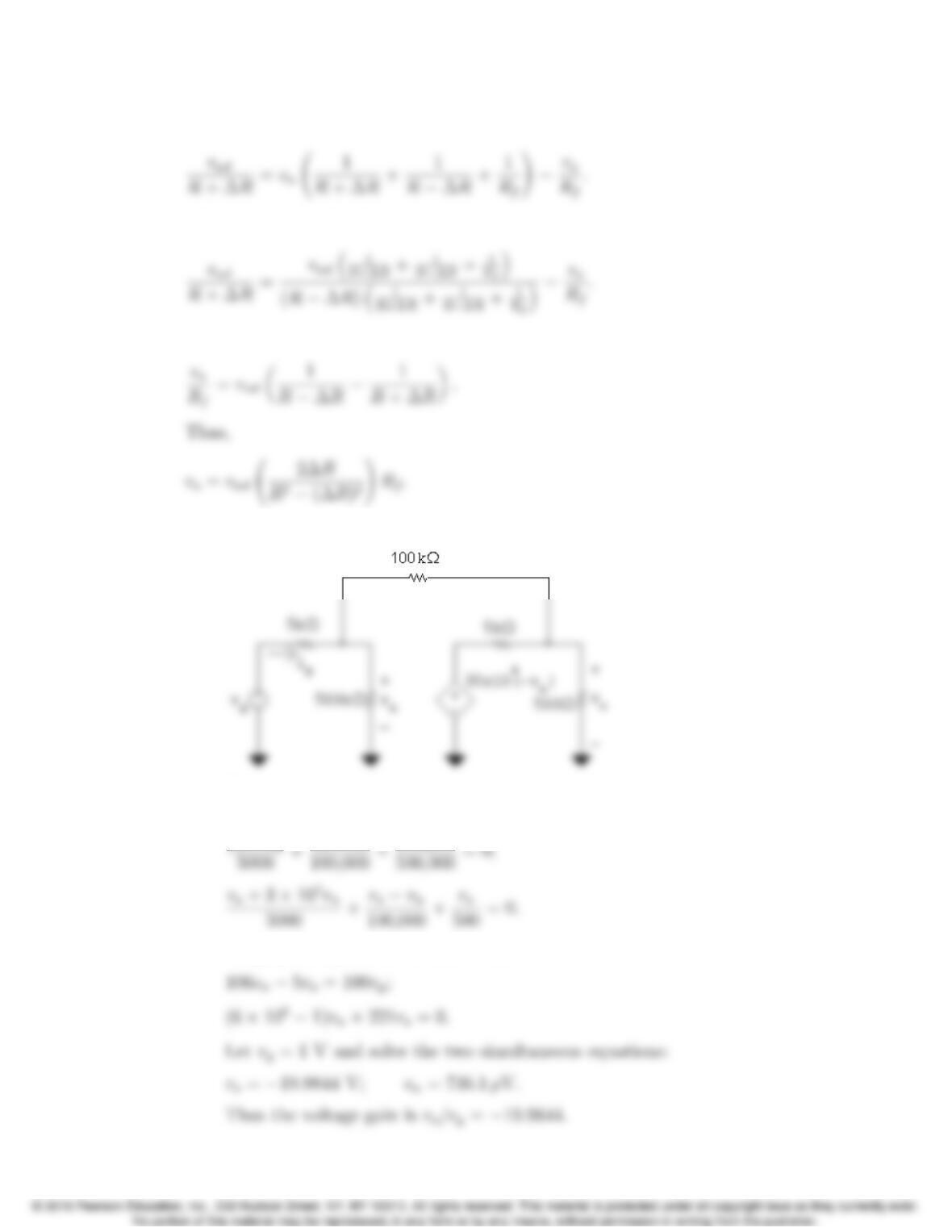
P 5.42 [a] p16 kΩ=(320 ⇥103)2
(16 ⇥103)=6.4µW.
[d] Yes, the operational amplifier serves several useful purposes:
•First, it enables the source to control 16 times as much power
5–28 CHAPTER 5. The Operational Amplifier
P 5.43 From Eq. 5.28,
Substituting Eq. 5.30 for vp=vn:
Rearranging,
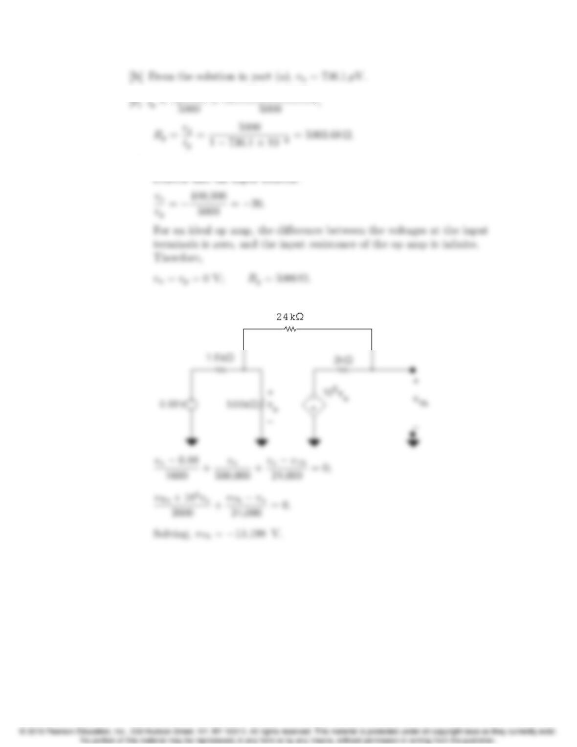
P 5.44 [a] Replace the op amp with the model from Fig. 5.18:
Write two node voltage equations, one at the left node, the other at the
right node:
vnvg
Simplify and place in standard form:
Problems 5–29
[d] For an ideal op amp, the voltage gain is the ratio between the feedback
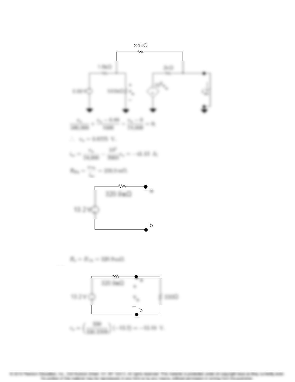
P 5.45 [a]
5–30 CHAPTER 5. The Operational Amplifier
Short-circuit current calculation:
[b] The output resistance of the inverting amplifier is the same as the
Th´evenin resistance, i.e.,
[c]
Problems 5–31
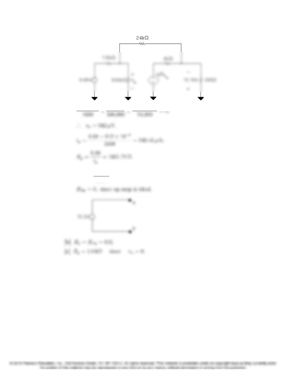
vn0.88
P 5.46 [a] vTh =24,000
1600 (0.88) = 13.2 V;
5–32 CHAPTER 5. The Operational Amplifier
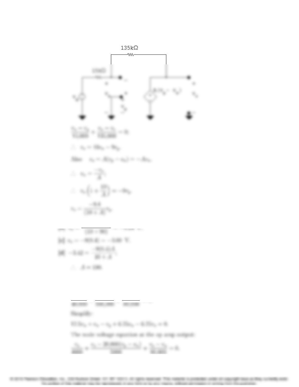
P 5.47 [a]
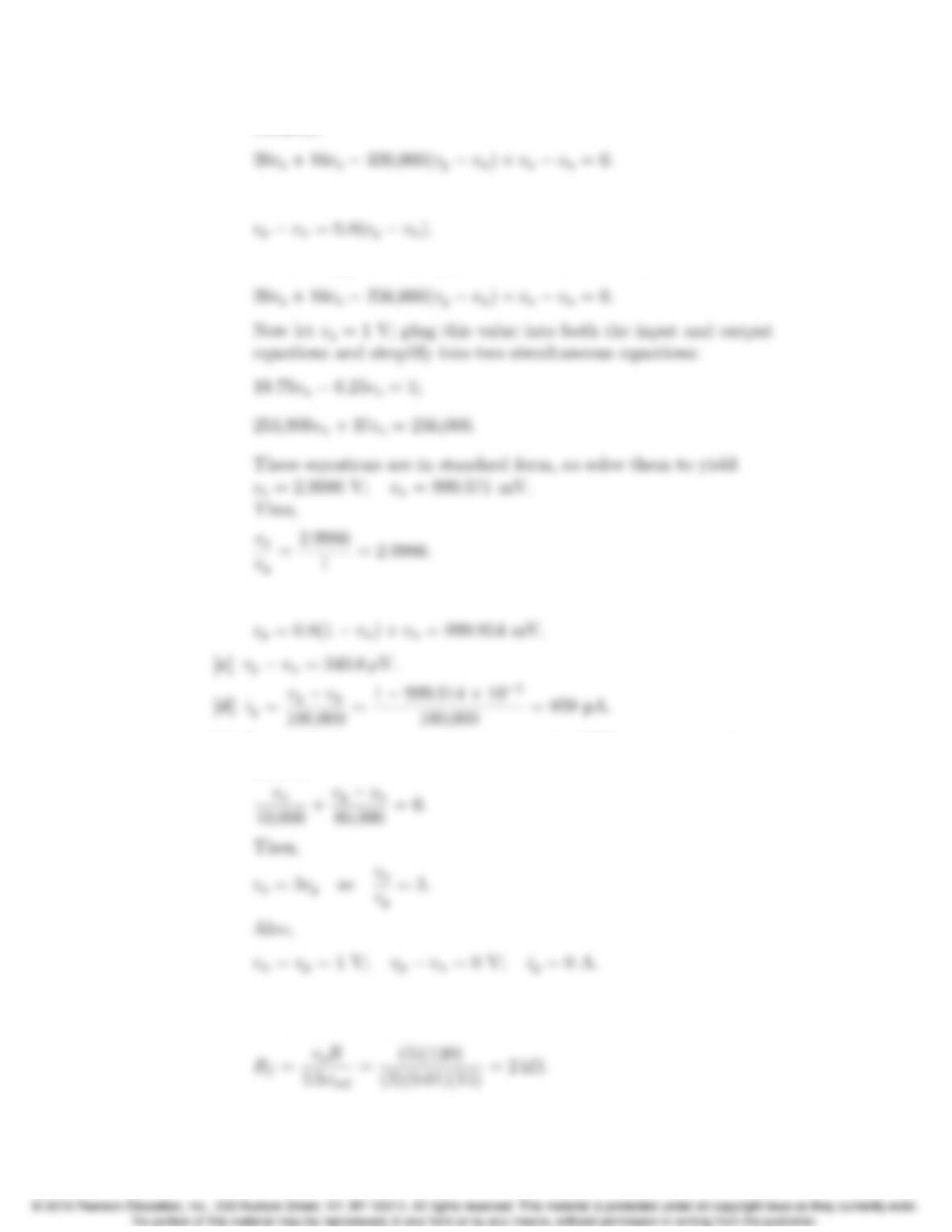
P 5.48 [a] Replace the op amp with the model shown in Fig. 5.18. The node voltage
equation at the inverting input:
vn
Problems 5–33
Simplify:
From the input,
Substituting into the equation written at the output,
[b] From part (a), vn= 999.571 mV. Use this value to solve for vp:
[e] For an ideal op amp, vn=vp=vg, so the KVL equation at the inverting
node is
P 5.49 [a] Use the approximation for Eq. 5.31 to solve for Rf; note that since we are
using 1% strain gages, ∆= 0.01:
5–34 CHAPTER 5. The Operational Amplifier
[b] Now solve for ∆given vo= 50 mV:
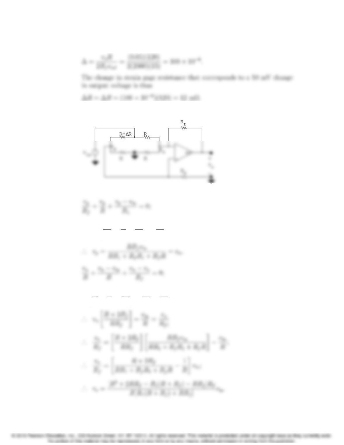
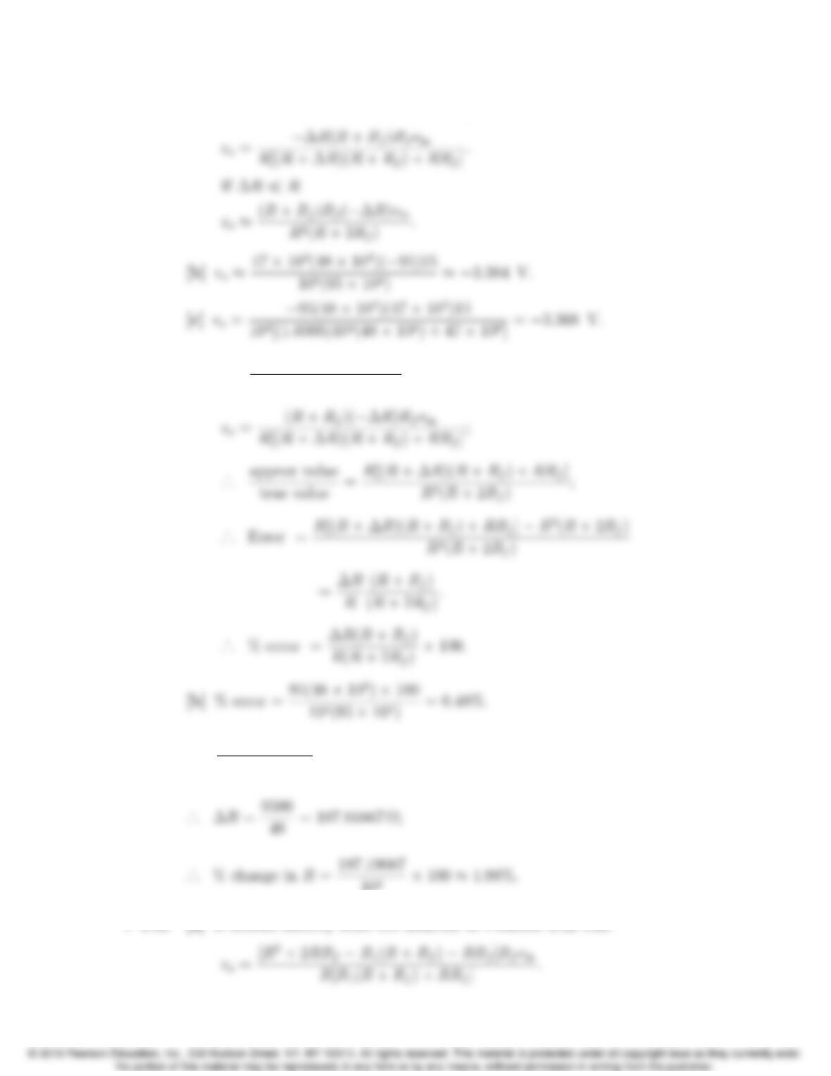
P 5.50 [a]
Let R1=R+∆R
·
.. v
p“1
Rf
+1
R+1
R1#=vin
R1
;
vn“1
R+1
R+1
Rf#vo
Rf
=vin
R;
Problems 5–35
Now substitute R1=R+∆Rand get
P 5.51 [a] vo⇡(R+Rf)Rf(∆R)vin
R2(R+2Rf);
P 5.52 1 = ∆R(48 ⇥104)
104(95 ⇥104)⇥100;
104⇥100 ⇡1.98%.
5–36 CHAPTER 5. The Operational Amplifier
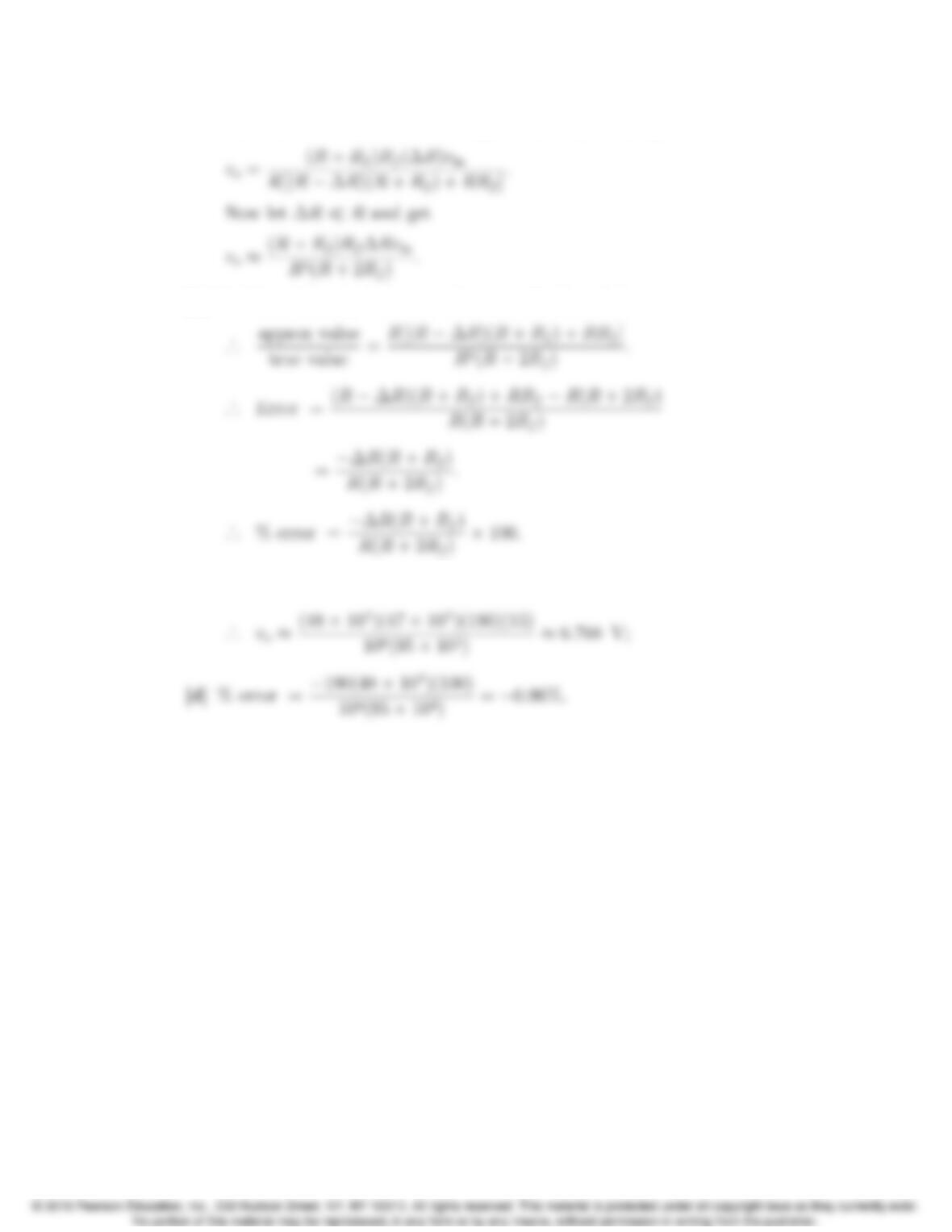
Now R1=R∆R. Substituting into the expression gives
[b] It follows directly from the solution to Problem 5.50 that
[c] R∆R= 9810 Ω·
.. ∆R= 10,000 9810 = 190 Ω;