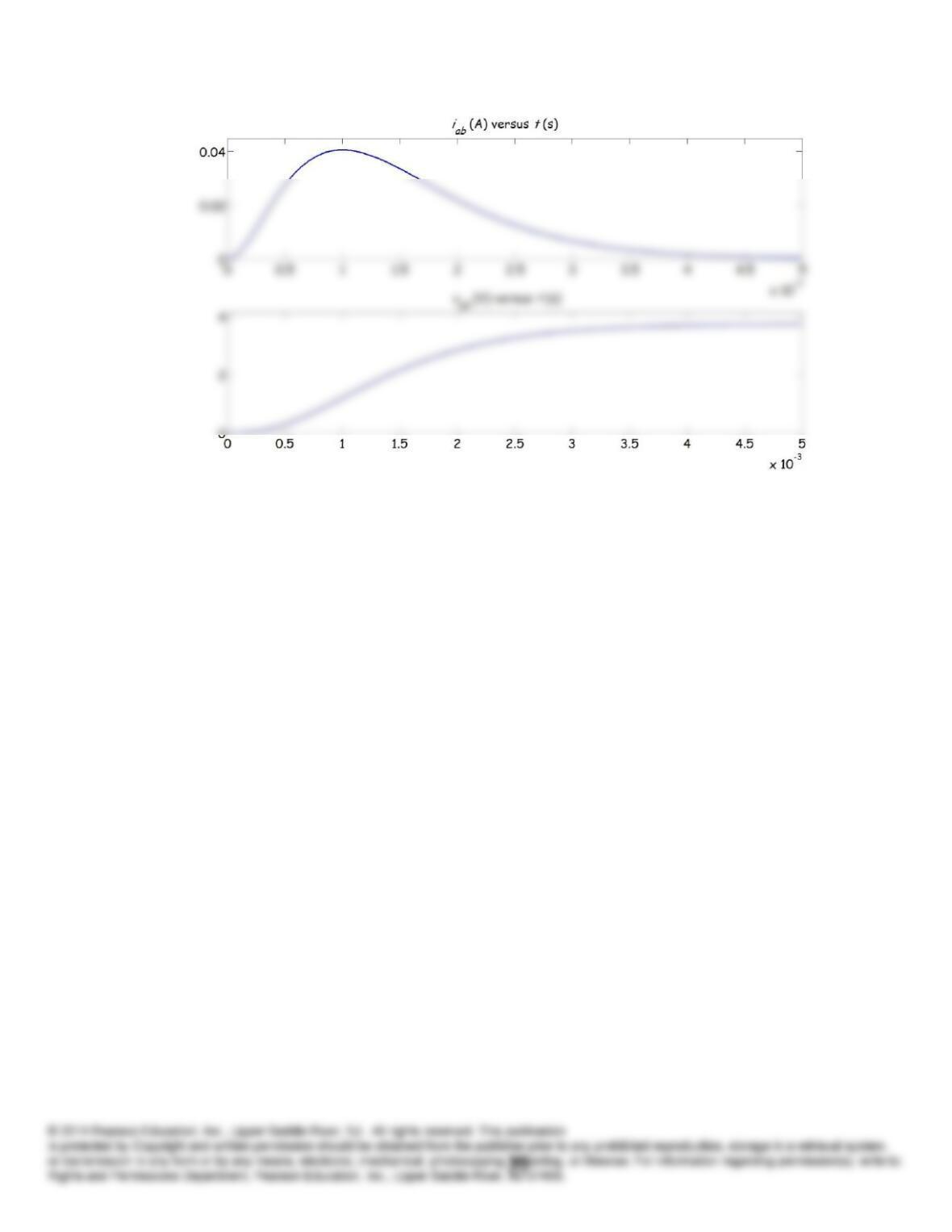
P3.46
1
0
10
1
t
LLL idttv
L
ti
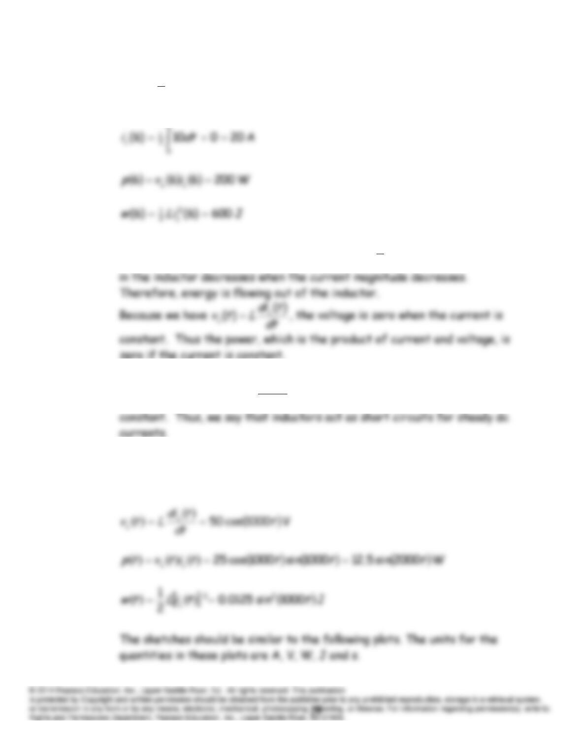
P3.47 Because the energy stored in an inductor is
2
2
1
Liw
, the energy stored
P3.48 Because we have
dt
tdi
Ltv L
L
)(
)(
, the voltage is zero when the current is
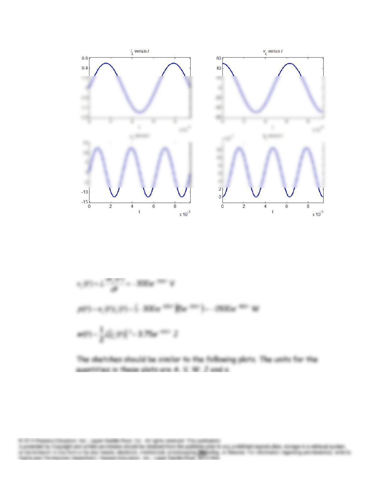
P3.49
H 1.0
L
A 1000sin5.0
ttiL
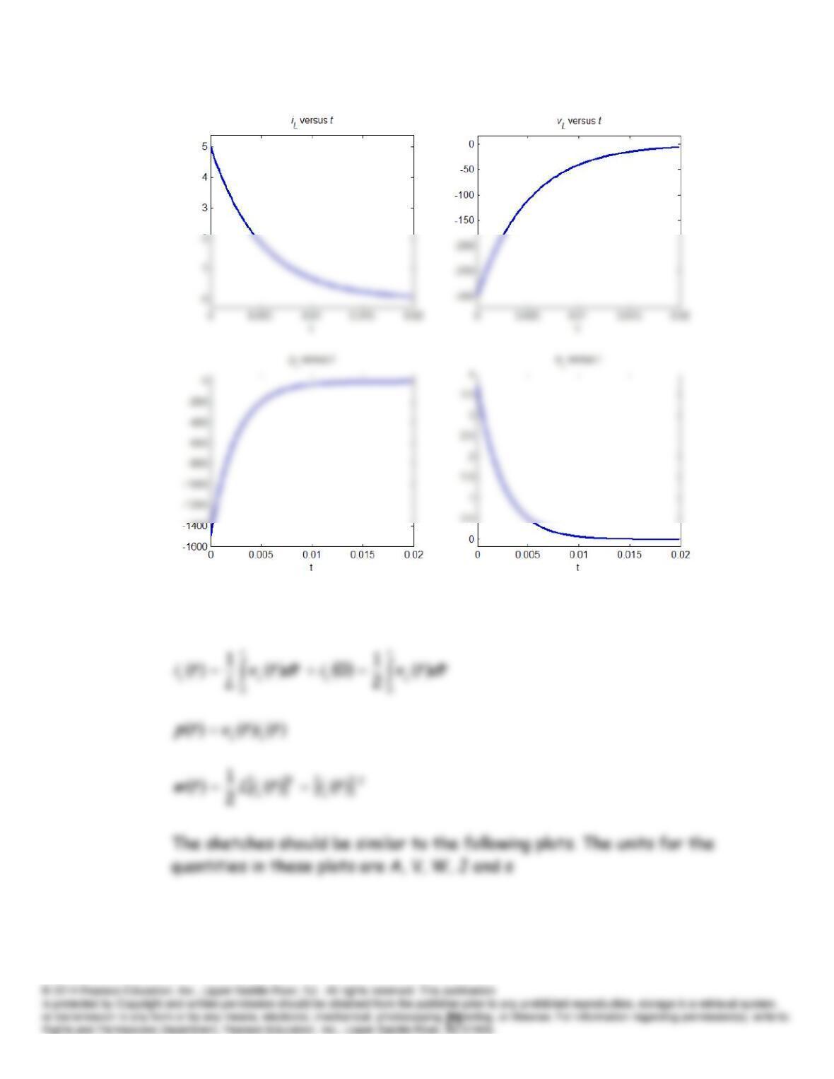
P3.50
H 3.0
L
t
Leti
200
5
P3.51
H 2
L
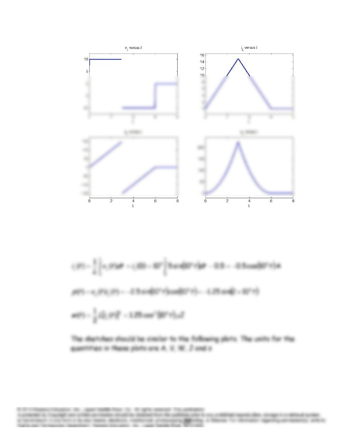
P3.52
H 10 μ
L
ttv L
6
10sin5
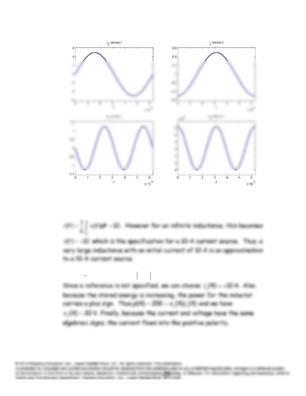
P3.53 For an inductor with an initial current of 10 A, we have
P3.54
A 10)4(J 100)4()4( 2
2
1
LL iLiw
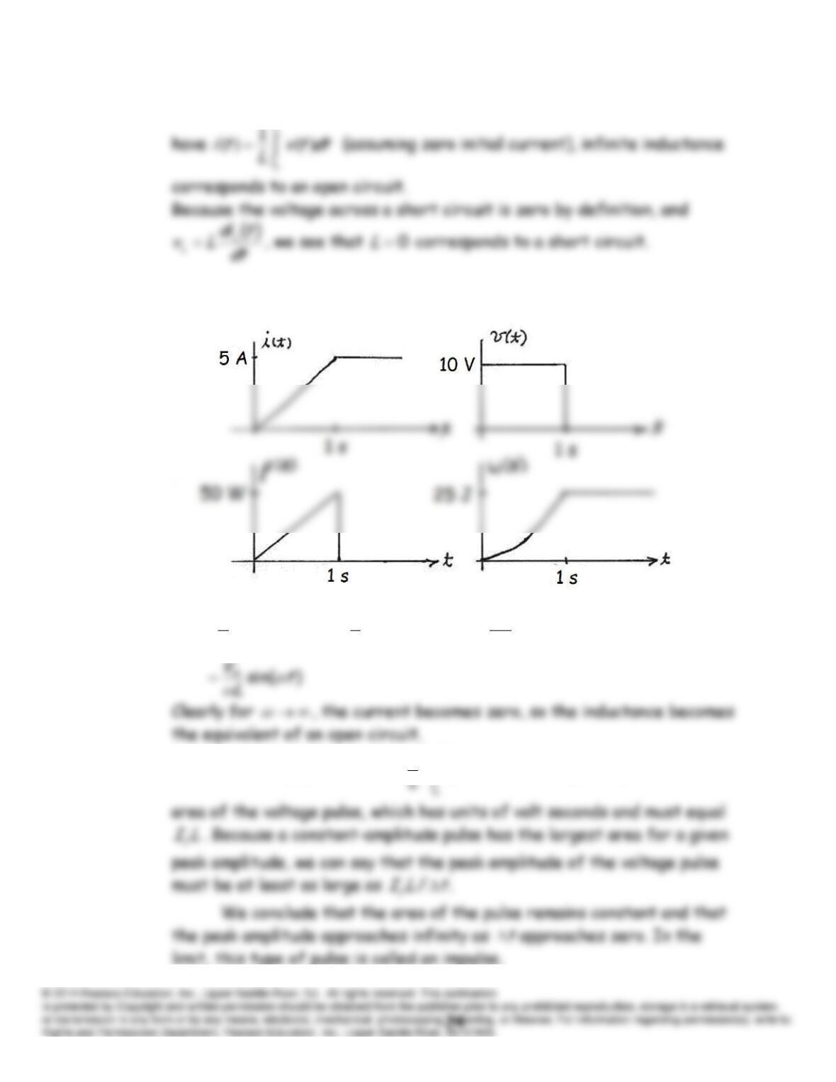
P3.55 Because the current through an open circuit is zero by definition, and we
P3.56
P3.57
)0sin()sin()cos(
1
0
1
00
t
L
V
dttV
L
idttv
L
ti m
t
m
t
P3.58 We can write
tt
L
f
Ldttv
Itti
0
1
0
. The integral represents the
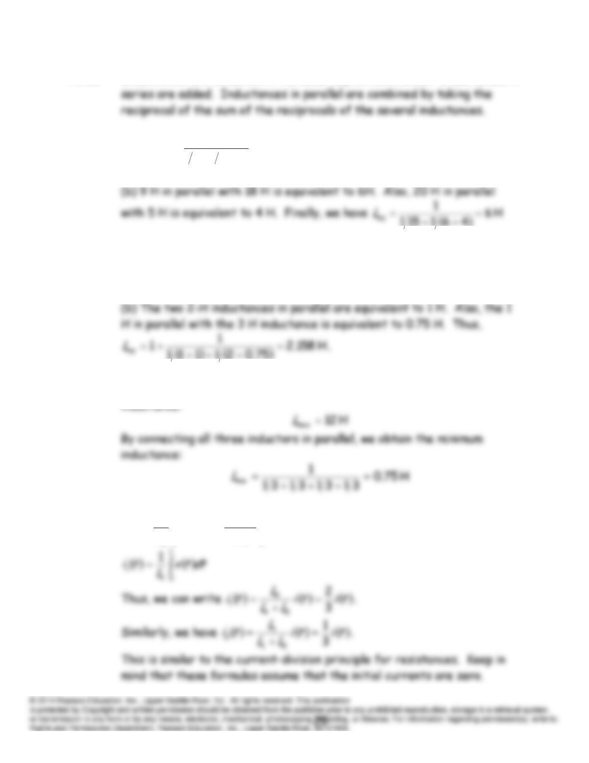
P3.59 Inductances are combined in the same way as resistances. Inductances in
P3.60* (a)
H 3
21161
1
1
eq
L
P3.61 (a) The 2 H inductors and 0.5 H inductor have no effect because they
are in parallel with a short circuit. Thus,
H 1
eq
L
.
P3.62 If all four inductors are connected in series, we obtain the maximum
P3.63*
t t
eq
dttv
LL
LL
dttv
L
ti
0 0
21
21
1
P3.64 Ordinarily, negative inductance is not practical. Thus, adding inductance
in series always increases the equivalent inductance. However, placing
P3.65 Ordinarily, negative inductance is not practical. Thus, adding inductance
in series always increases the equivalent inductance. However, placing
P3.66
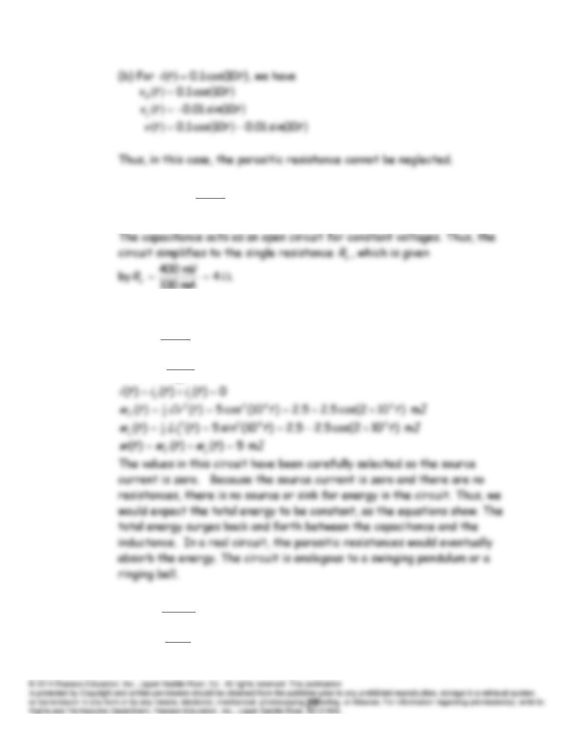
P3.67 (a)
tRitv
5
10cos1.0
P3.68 Because
0
)(
dt
tdi
Lv L
L
for currents that are constant in time, we
conclude that the inductance behaves as a short circuit for dc currents.
P3.69
)10cos(100)]10[cos(101010
)(
)( 4443
tt
dt
tdi
Ltv L
V
)10sin(
)(
)( 4
t
dt
tdv
CtiC
A
P3.70
)1000sin(10)]1000sin([10004010250
)(
)( 6
tt
dt
tdv
Cti C
A
)1000cos(40
)(
)(
t
dt
tdi
Ltv L
V
0)()()(
tvtvtv L
C
P3.71 When a time-varying current flows in a coil, a time-varying magnetic field
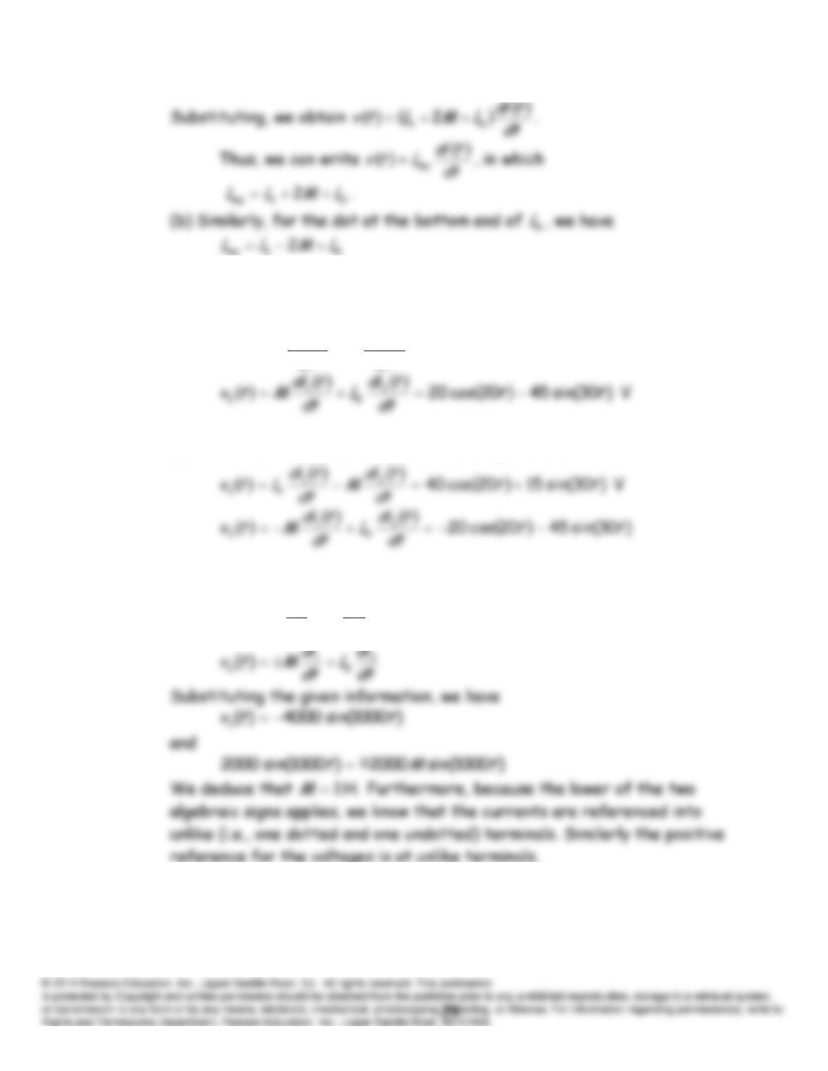
P3.72* (a)
As in Figure 3.23a, we can write
tdi
M
tdi
Ltv
21
11
2
L
P3.73 (a) Refer to Figures 3.23 and P3.73. For the dots as shown in Figure
P3.73, we have
)30sin(1520cos40
21
11
tt
dt
tdi
M
dt
tdi
Ltv
V
(b) With the dot moved to the bottom of
2
L
, we have
)30sin(1520cos40
21
11
tt
dt
tdi
M
dt
tdi
Ltv
P3.74 In general, we have
dt
di
M
dt
di
Ltv
21
11
)(
P3.75 With a short circuit across the terminals of the second coil, we have
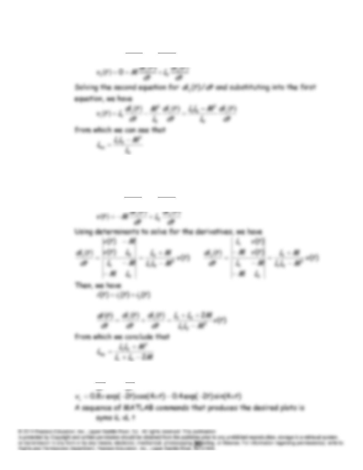
dt
tdi
M
dt
tdi
Ltv
21
11
P3.76 Because of the parallel connection, we have
)()()( 21
tvtvtv
and the
equations for the mutually coupled inductors become
dt
tdi
M
dt
tdi
Ltv
21
1
P3.77
)4sin()2exp(2.0
tt
d
di
Lv L
L
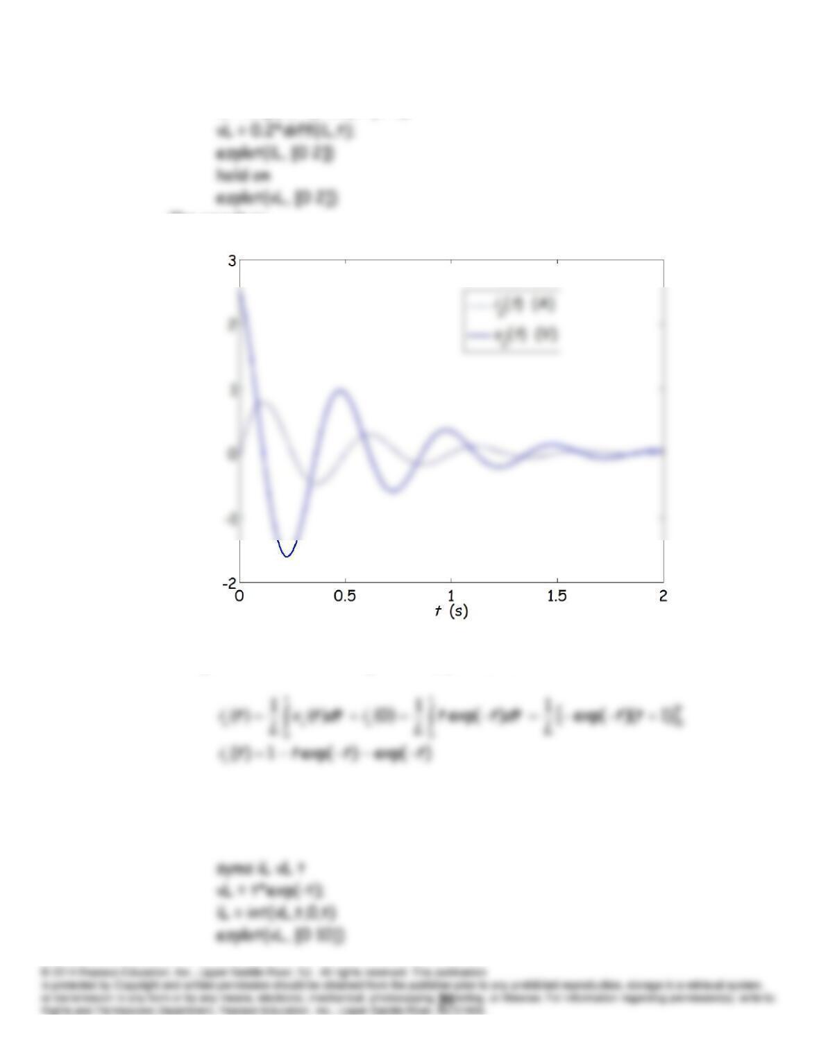
iL = exp(-2*t)*sin(4*pi*t);
The result is:
P3.78 Using either tables or integration by parts, we have
A sequence of MATLAB commands to verify our result for
iL
(
t
) and obtain
the desired plots is
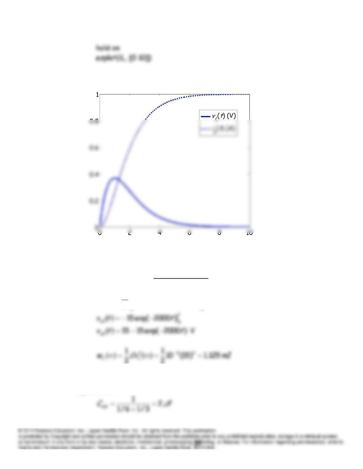
The result is:
Practice Test
T3.1
tt
C
abab dttvdtti
C
tv
5
)2000exp(3.0100
1
T3.2 The 6-
F and 3-
F capacitances are in series and have an equivalent
capacitance of
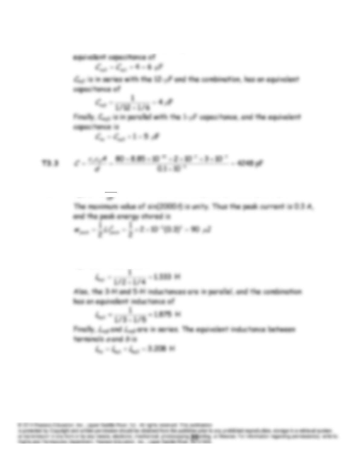
C
eq1 is in parallel with the 4-
F capacitance, and the combination has an
T3.4
)2000cos(2.1)2000cos(20003.0102)( 3
tt
di
Ltv ab
ab
V
T3.5 The 2-H and 4-H inductances are in parallel and the combination has an
equivalent inductance of
T3.6 For these mutually coupled inductances, we have
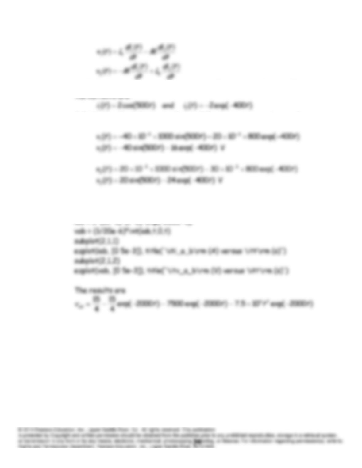
in which the currents are referenced into the positive polarities. Thus
the currents are
Substituting the inductance values and the current expressions we have
T3.7 One set of commands is
syms vab iab t
iab = 3*(10^5)*(t^2)*exp(-2000*t);