CHAPTER 2
Exercises
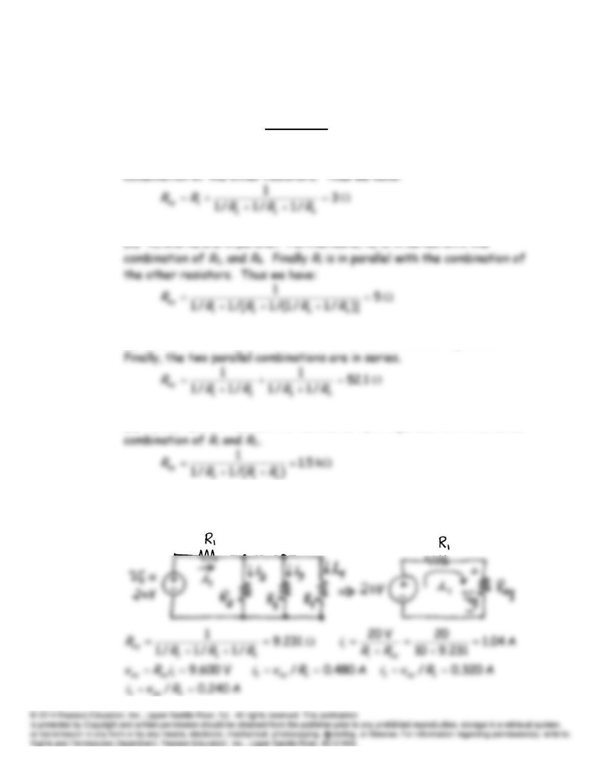
E2.1 (a)
R
2
, R
3
,
and
R
4 are in parallel. Furthermore
R
1 is in series with the
(b)
R
and
R
R
(c)
R
1
and
R
2 are in parallel. Furthermore,
R
3
,
and
R
4 are in parallel.
(d)
R
1
and
R
2 are in series. Furthermore,
R
3 is in parallel with the series
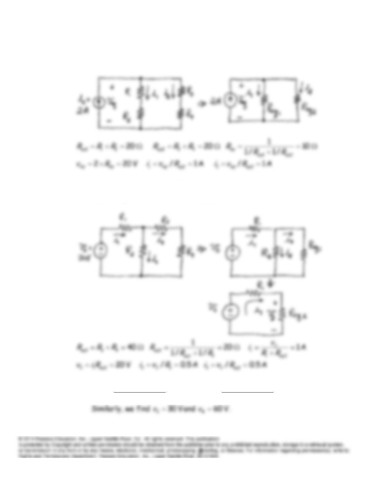
E2.2 (a) First we combine
R
2,
R
3
,
and
R
4 in parallel. Then
R
1 is in series with
the parallel combination.
(b)
R
1
and
R
2 are in series. Furthermore,
R
3
,
and
R
4 are in series.
Finally, the two series combinations are in parallel.
(c)
R
3
,
and
R
4 are in series. The combination of
R
3
and
R
4 is in parallel
with
R
2. Finally the combination of
R
2,
R
3
,
and
R
4 is in series with
R
1.
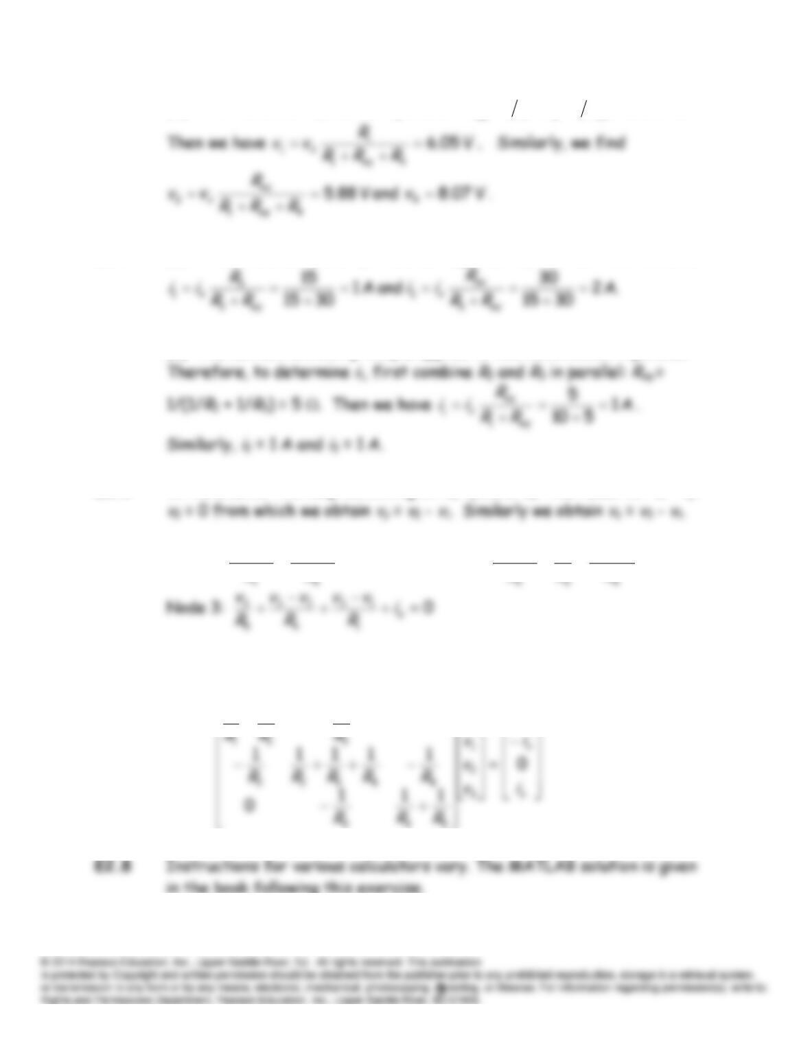
E2.3 (a)
V 10
4321
1
1
RRRR
R
vv s
.
V 20
4321
2
2
RRRR
R
vv s
.
(b) First combine
R
2 and
R
3 in parallel:
. 917.2)1/1(1 32
RRReq
E2.4 (a) First combine
R
1 and
R
2 in series:
Req
=
R
1 +
R
2 = 30 . Then we have
(b) The current division principle applies to two resistances in parallel.
E2.5 Write KVL for the loop consisting of
v
1,
vy
, and
v
2. The result is –
v
1 –
vy
+
E2.6 Node 1:
a
i
R
vv
R
vv
21
31
Node 2:
0
32
2
12
R
vv
R
v
R
vv
E2.7 Following the step-by-step method in the book, we obtain
0
111
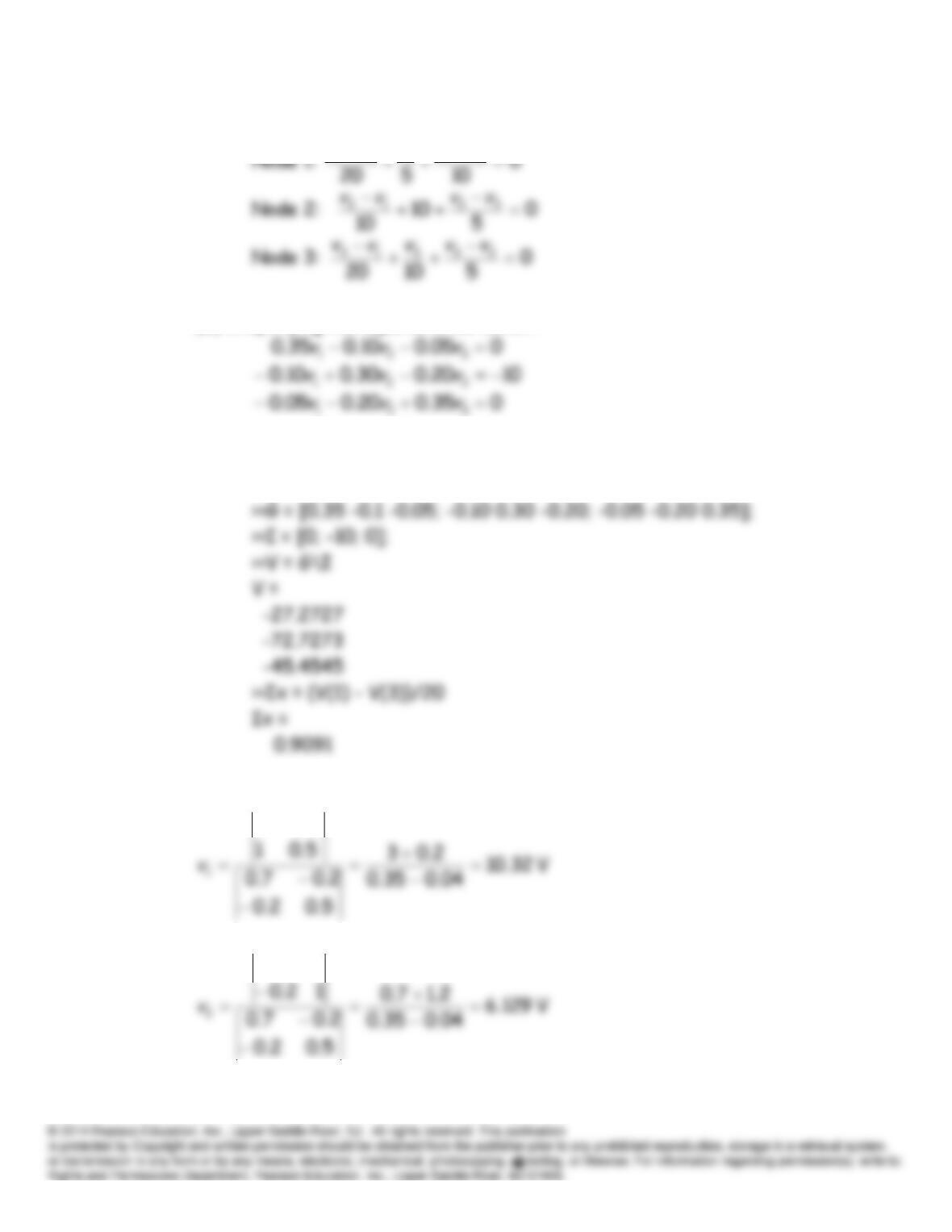
E2.9 (a) Writing the node equations we obtain:
211
31
vvv
vv
(b) Simplifying the equations we obtain:
(c) and (d) Solving using Matlab:
>>clear
E2.10 Using determinants we can solve for the unknown voltages as follows:
2.06
67.0
Many other methods exist for solving linear equations.
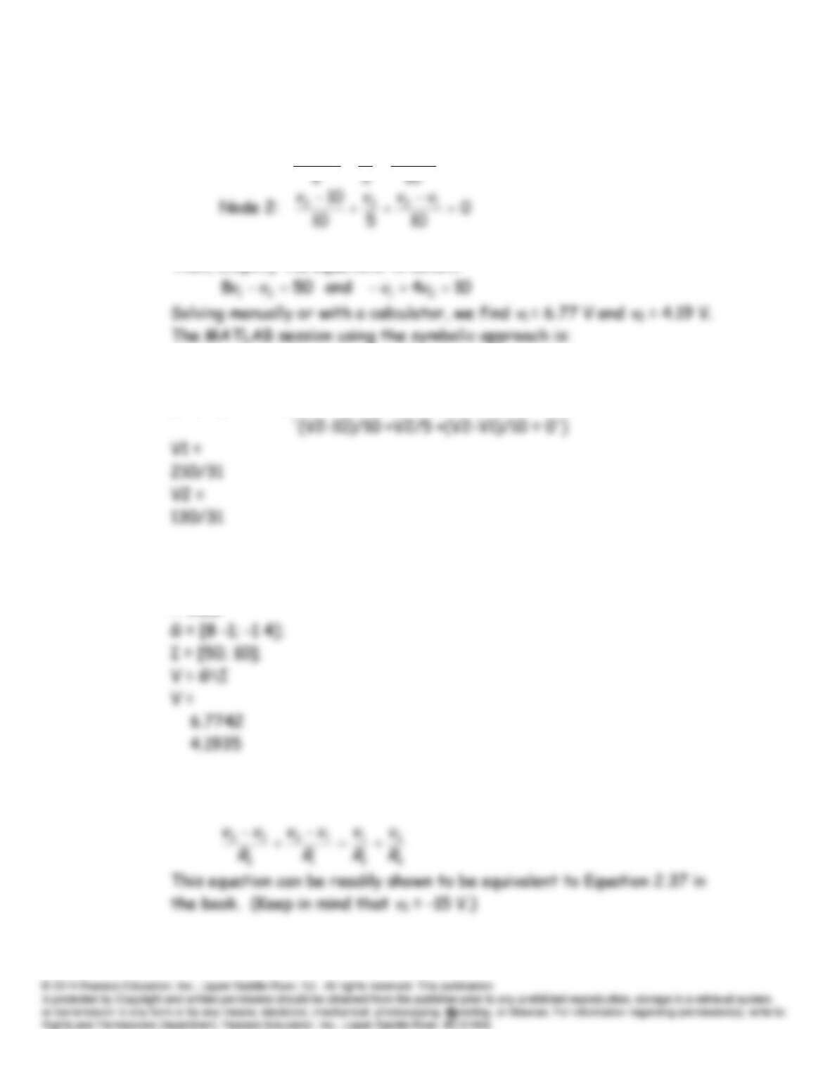
E2.11 First write KCL equations at nodes 1 and 2:
Node 1:
0
10 2111
vvvv
Then, simplify the equations to obtain:
>> clear
[V1,V2] = solve(‘(V1-10)/2+(V1)/5 +(V1 – V2)/10 = 0′ , …
Next, we solve using the numerical approach.
>> clear
E2.12 The equation for the supernode enclosing the 15-V source is:
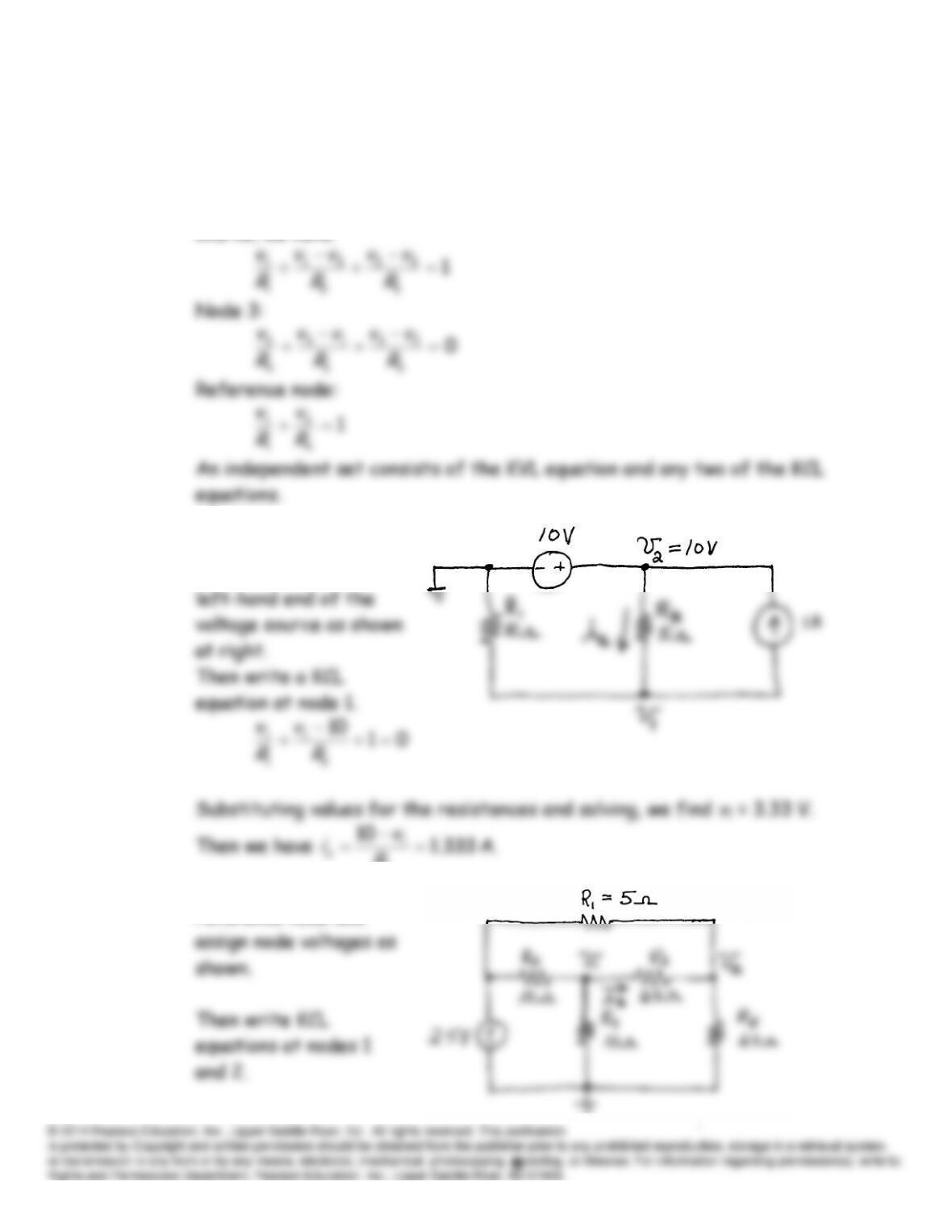
E2.13 Write KVL from the reference to node 1 then through the 10-V source to
node 2 then back to the reference node:
010 21
vv
Then write KCL equations. First for a supernode enclosing the 10-V
source, we have:
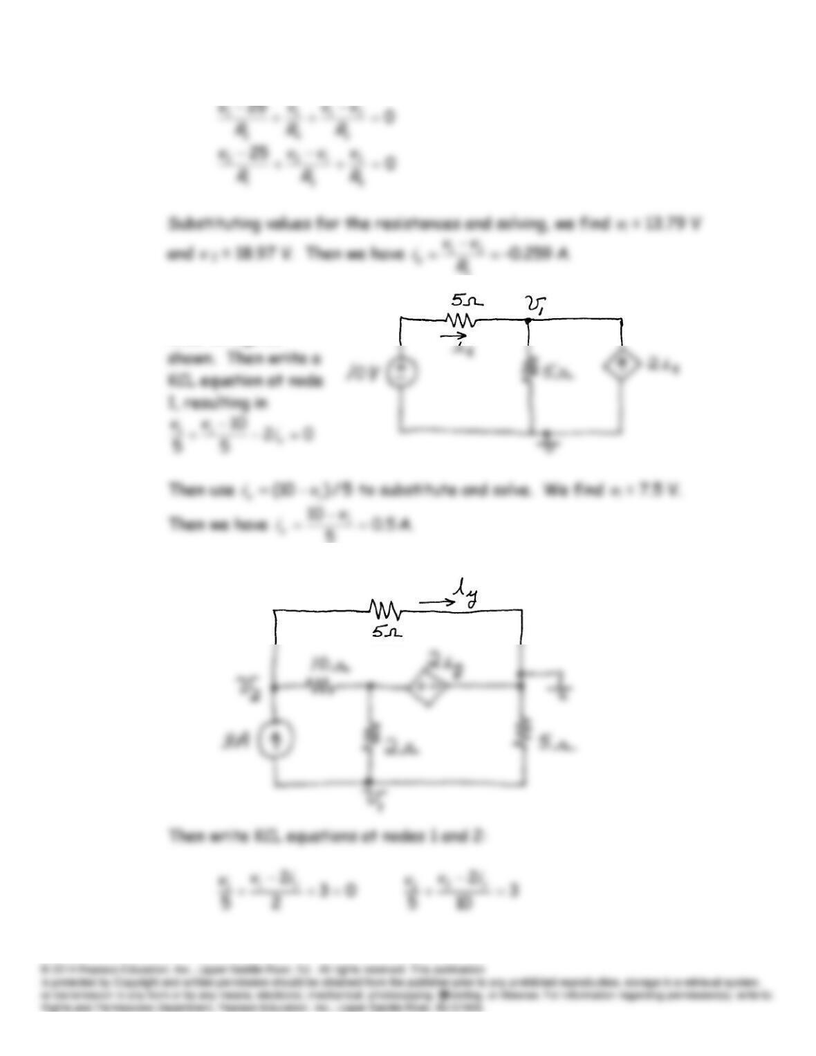
E2.14 (a) Select the
reference node at the
2
R
(b) Select the
reference node and
3
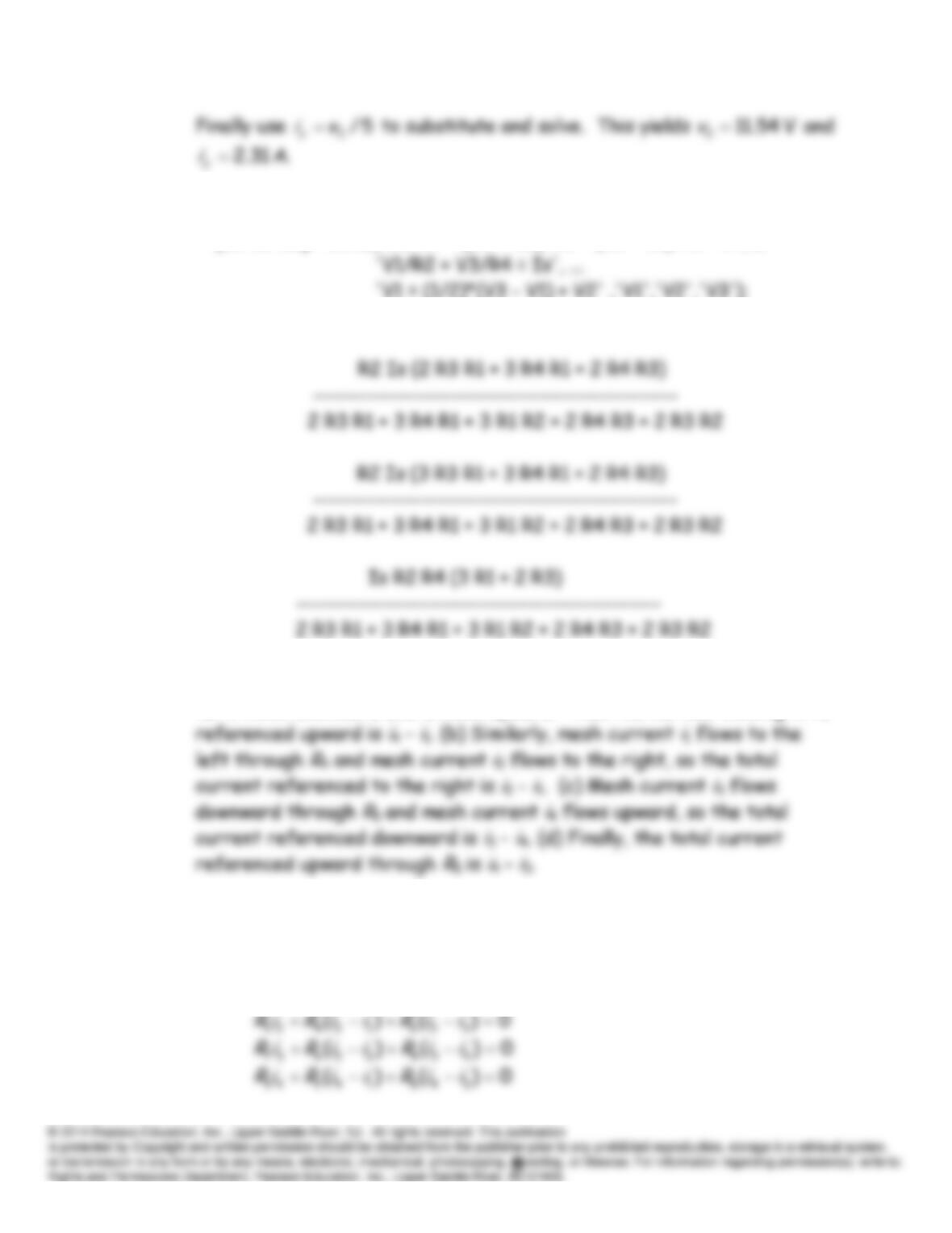
E2.15 (a) Select the
reference node and
node voltage as
(b) Choose the reference node and node voltages shown:
E2.16 >> clear
>> [V1 V2 V3] = solve(‘V3/R4 + (V3 – V2)/R3 + (V3 – V1)/R1 = 0′, …
‘V1 = (1/2)*(V3 – V1) + V2′ ,’V1′,’V2′,’V3’);
>> pretty(V1), pretty(V2), pretty(V3)
E2.17 Refer to Figure 2.33b in the book. (a) Two mesh currents flow through
R
2:
i
1 flows downward and
i
4 flows upward. Thus the current flowing in
R
2
E2.18 Refer to Figure 2.33b in the book. Following each mesh current in turn,
we have
0)()( 21441211
A
viiRiiRiR
In matrix form, these equations become
0)(
1
24421
A
v
i
RRRRR
E2.19 We choose the mesh currents as shown:
Then, the mesh equations are:
Simplifying and solving these equations, we find that
A 10
1
i
and
To solve by node voltages, we select the reference node and node voltage
E2.20 First, we assign the mesh currents as shown.
Then we write KVL equations following each mesh current:
Simplifying and solving, we find that
i
1 = 2.194 A,
i
2 = 0.839 A, and
i
3 =
E2.21 Following the step-by-step process, we obtain
E2.22 Refer to Figure 2.39 in the book. In terms of the mesh currents, the
E2.23 Refer to Figure 2.40 in the book. First, for the current source, we have
Then, we write a KVL equation going around the perimeter of the entire
circuit:
E2.24 (a) As usual, we
select the mesh
currents flowing
clockwise around the
(b) As usual, we select
the mesh currents
E2.25 (a) KVL mesh 1:
0)(5510 211
iii
(b) First for the current
source, we have:
A 3
1
i
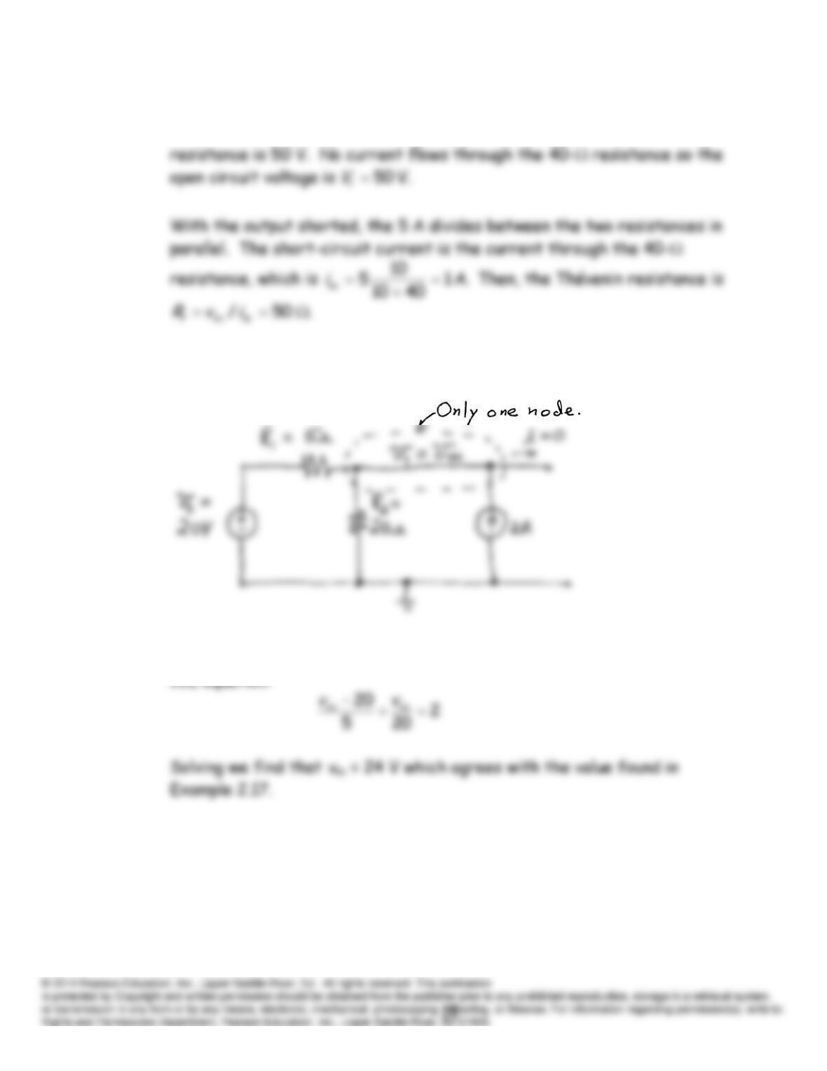
E2.26 Under open-circuit conditions, 5 A circulates clockwise through the
current source and the 10- resistance. The voltage across the 10-
E2.27 Choose the reference node at the bottom of the circuit as shown:
Notice that the node voltage is the open-circuit voltage. Then write a
E2.28 To zero the sources, the voltage sources become short circuits and the
current sources become open circuits. The resulting circuits are :
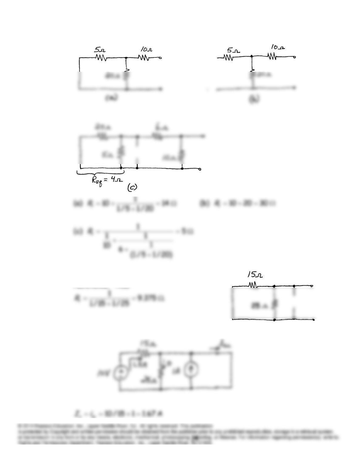
E2.29 (a) Zero sources to determine Thévenin
resistance. Thus
Then find short-circuit current:
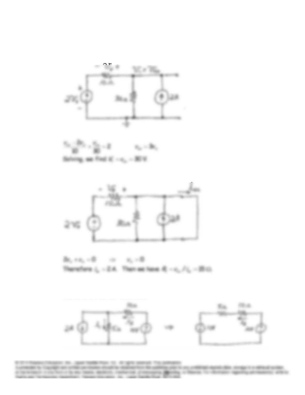
(b) We cannot find the Thévenin resistance by zeroing the sources,
because we have a controlled source. Thus, we find the open-circuit
voltage and the short-circuit current.
Now, we find the short-circuit current:
E2.30 First, we transform the 2-A source and the 5-Ω resistance into a voltage
source and a series resistance:
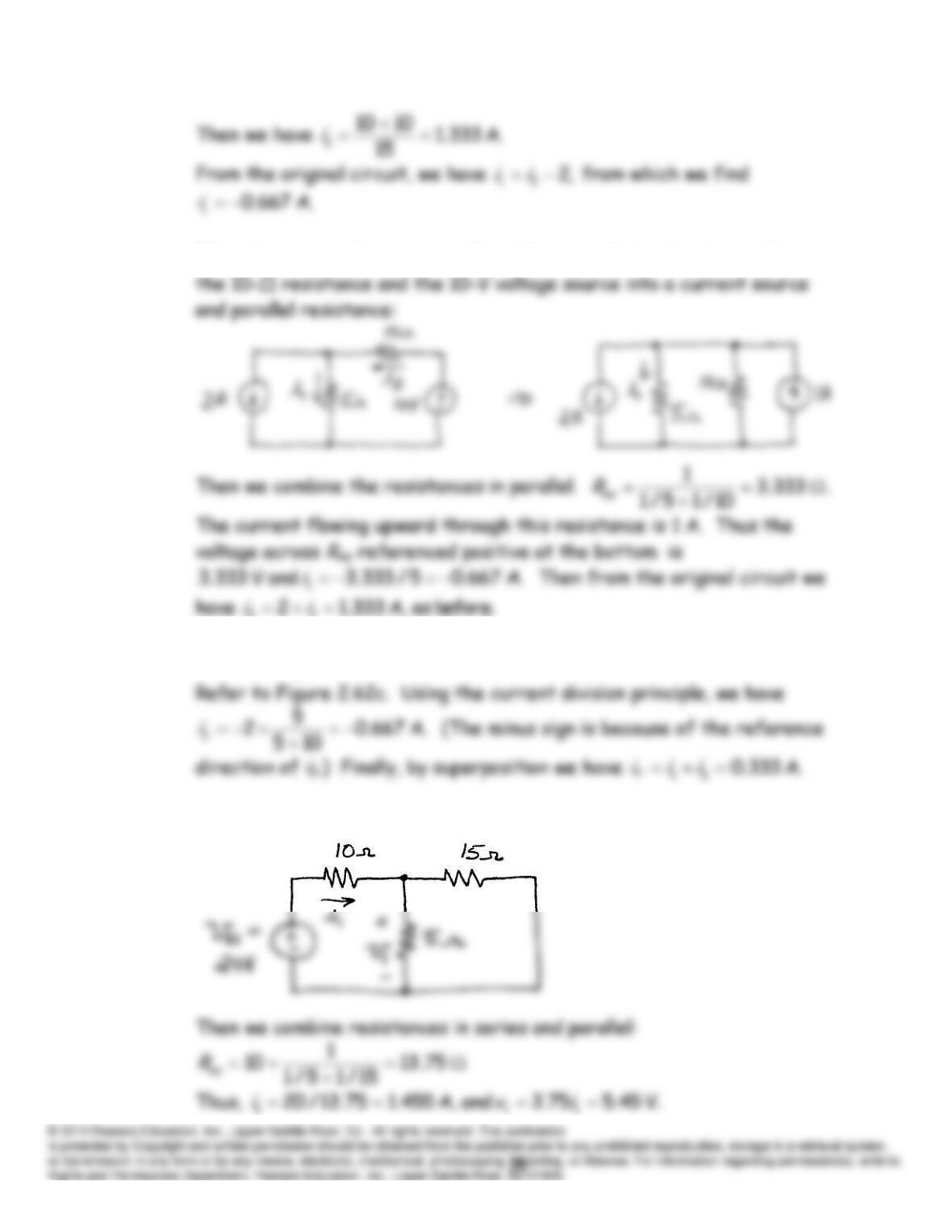
The other approach is to start from the original circuit and transform
E2.31 Refer to Figure 2.62b. We have
A. 115/15
1
i
E2.32 With only the first source active we have:
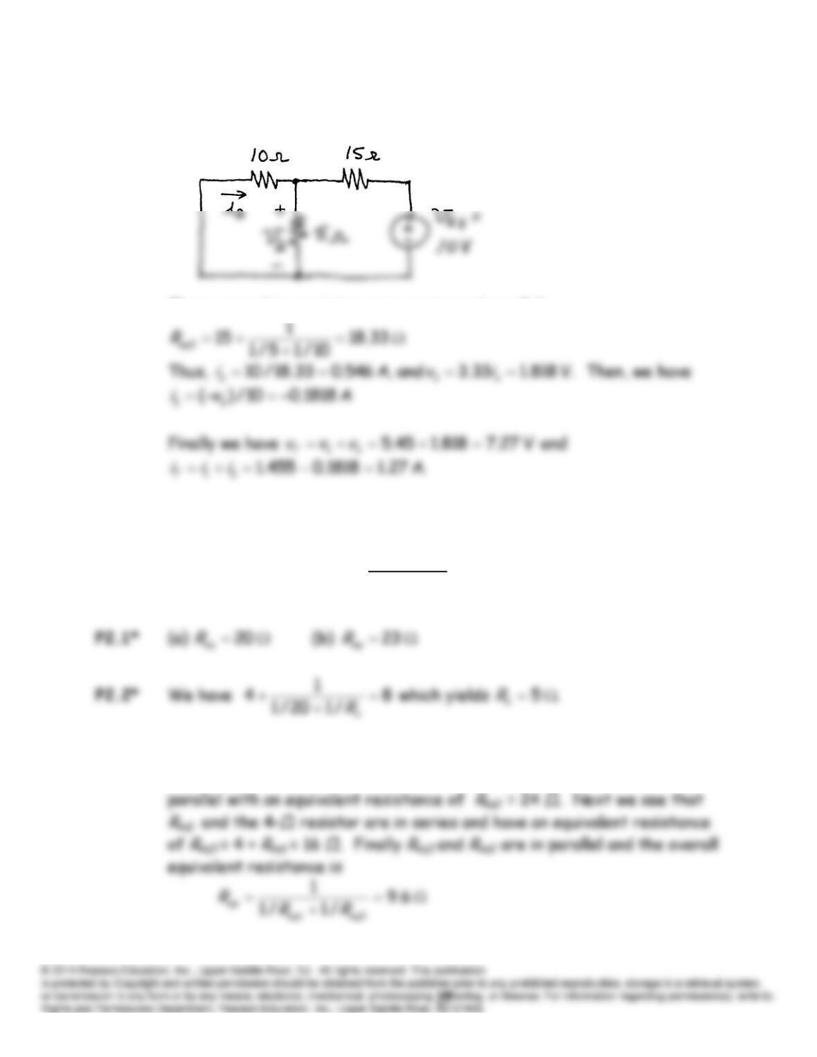
With only the second source active, we have:
Then we combine resistances in series and parallel:
Problems
P2.3* The 20-Ω and 30–Ω resistances are in parallel and have an equivalent
resistance of
R
eq1 = 12 Ω. Also the 40–Ω and 60–Ω resistances are in
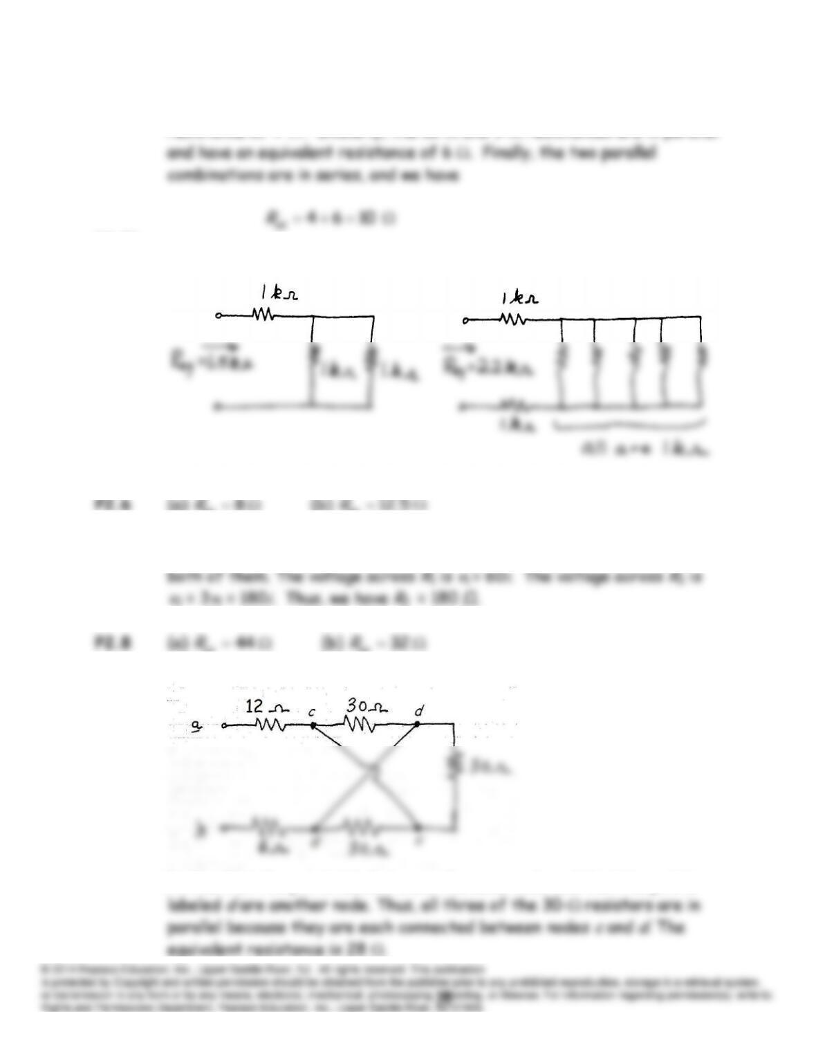
P2.4* The 12-
and 6-
resistances are in parallel having an equivalent
resistance of 4
. Similarly, the 18- and 9- resistances are in parallel
P2.5*
eq
eq
P2.7 Because the resistances are in series, the same current
i
flows through
eq
eq
(c)
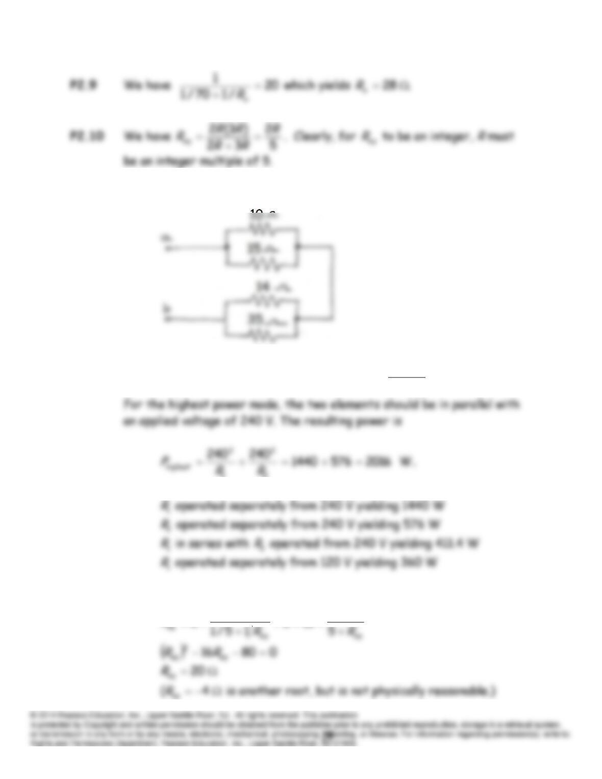
Notice that the points labeled
c
are the same node and that the points
P2.11
16
ab
R
P2.12 In the lowest power mode, the power is
9.102
120
21
2
RR
Plowest
W.
2
1
Some other modes and resulting powers are:
P2.13 Combining the resistances shown in Figure P2.13b, we have
eq
R
R
5
5
168
1
8
1000
1
1
P2.15 For operation at the lowest power, we have
21
2
120
180
RR
P
At the high power setting, we have
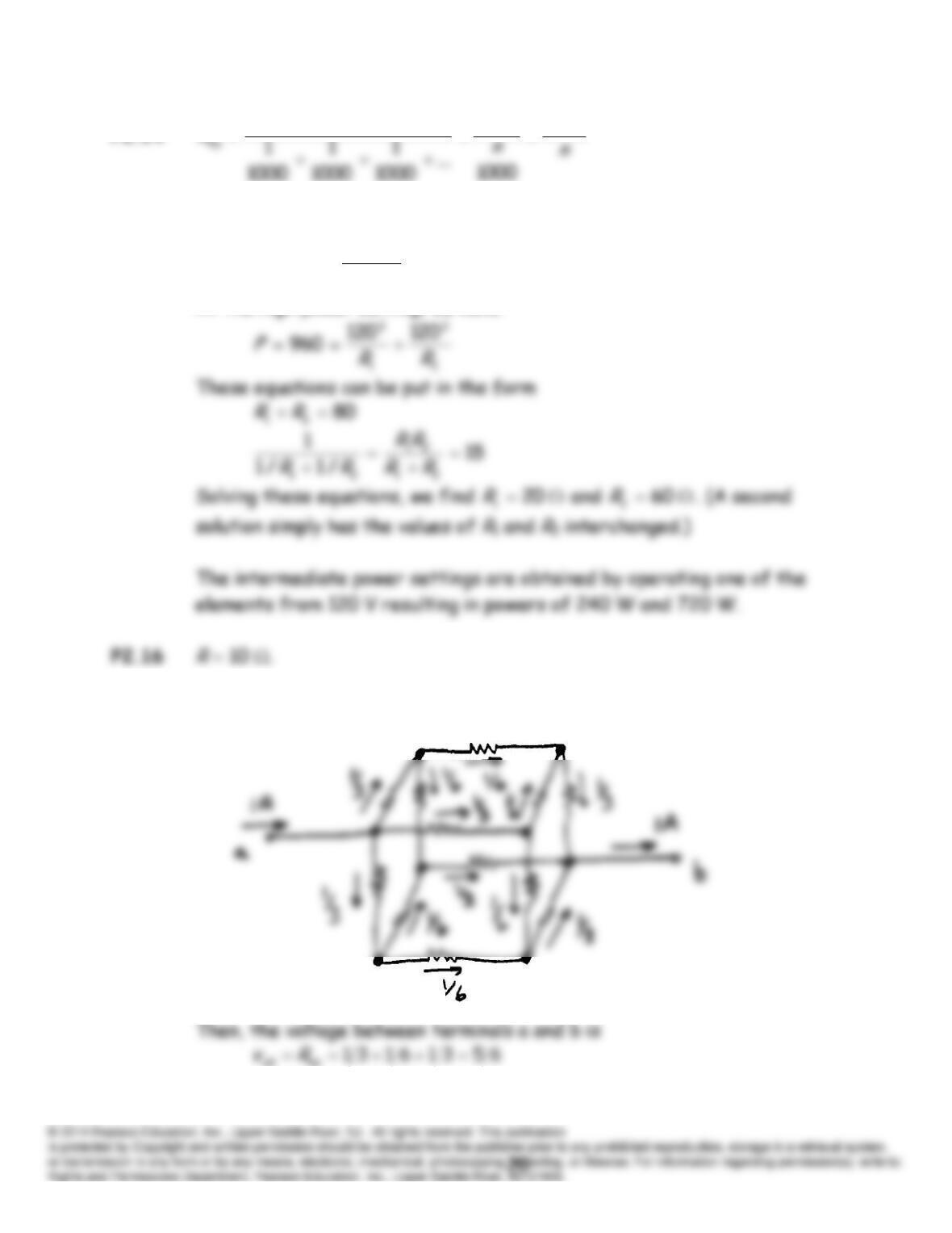
P2.17 By symmetry, we find the currents in the resistors as shown below: