P2.18 (a) For a series combination
1
Geq
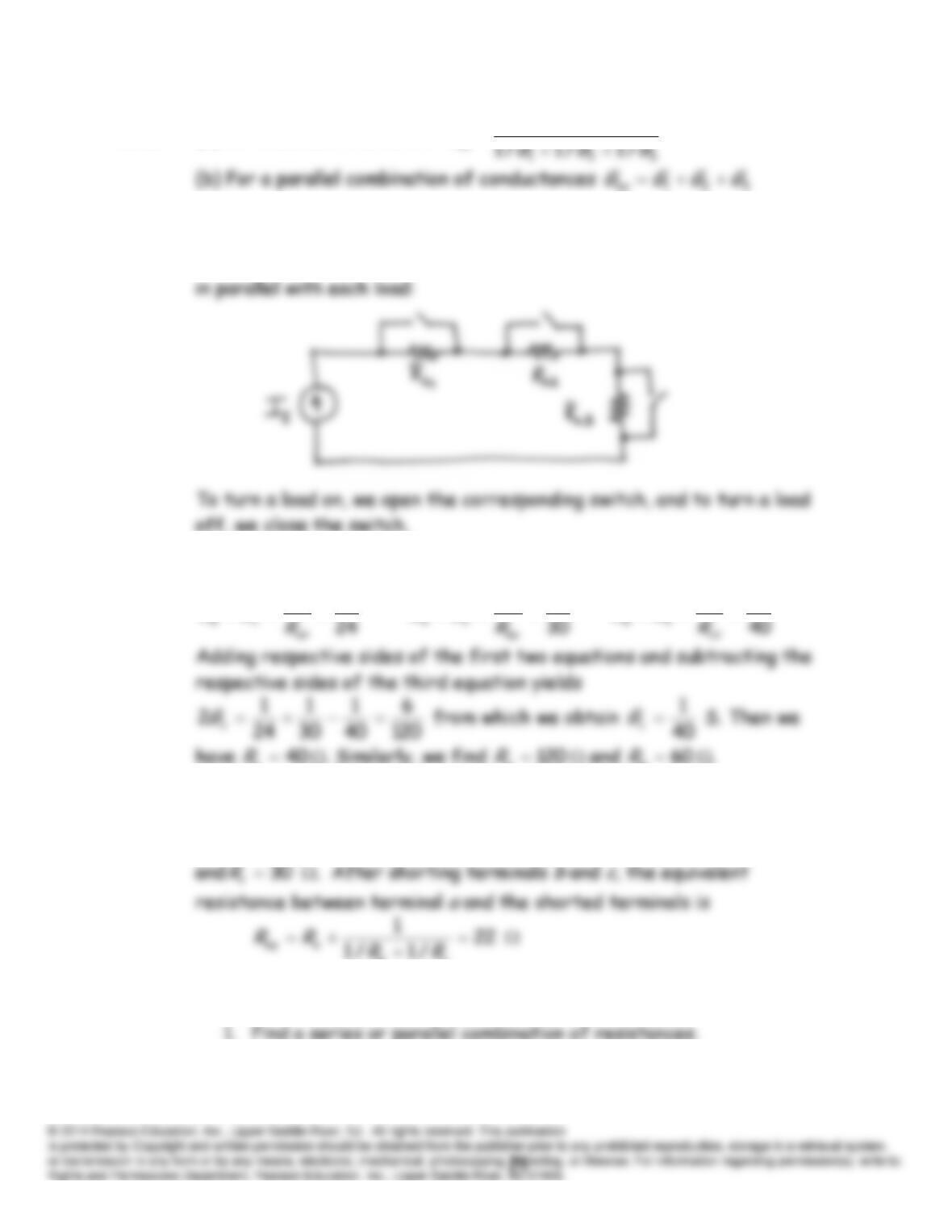
P2.19 To supply the loads in such a way that turning one load on or off does not
affect the other loads, we must connect the loads in series with a switch
P2.20 The equations for the conductances are
11
GG
11
GG
11
GG
c
a
b
P2.21 We have
,30
abb
aRRR
50
bc
c
bRRR
and
40
caca RRR
.
These equations can be solved to find that
10
a
R
,
20
b
R
,
c
c
b
P2.22 The steps in solving a circuit by network reduction are:
2. Combine them.
4. Solve for the currents and voltages in the final circuit. Transfer
5. Check to see that KVL and KCL are satisfied in the original
network.
P2.23*
A 1
10
1010
1
eq
R
i
P2.24*
75.3
15151
1
eq
R
V 5.7A 2
eqxRv
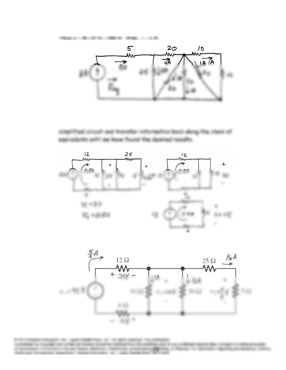
P2.25* Combining resistors in series and parallel, we find that the equivalent
P2.26* We combine resistances in series and parallel until the circuit becomes an
equivalent resistance across the voltage source. Then, we solve the
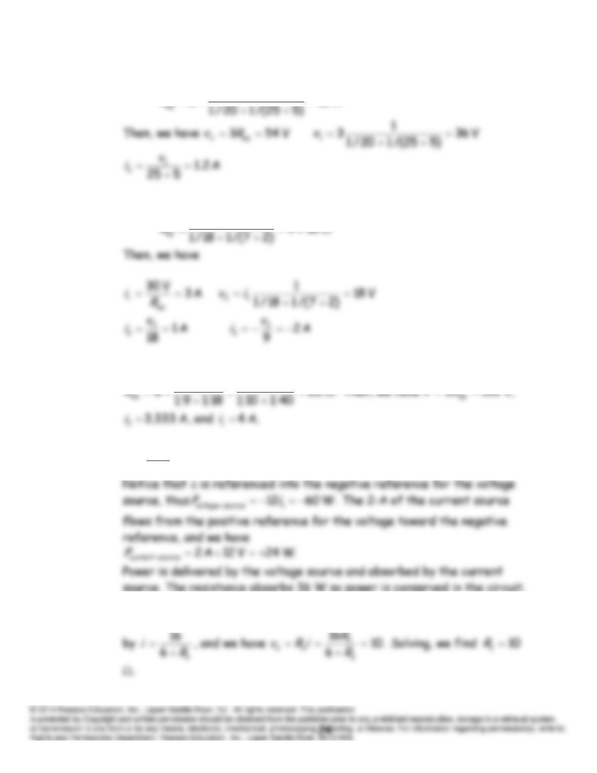
P2.27 Using Ohm’s and Kirchhoff’s laws, we work from right to left resulting in
P2.28 The equivalent resistance seen by the current source is
18
1
6
R
P2.29 The equivalent resistance seen by the voltage source is
1
P2.30 The equivalent resistance seen by the current source is
1
1
P2.31
A 3
4
V 12
2
i
A 52
21
ii
P2.32 With the switch open, the current flowing clockwise in the circuit is given
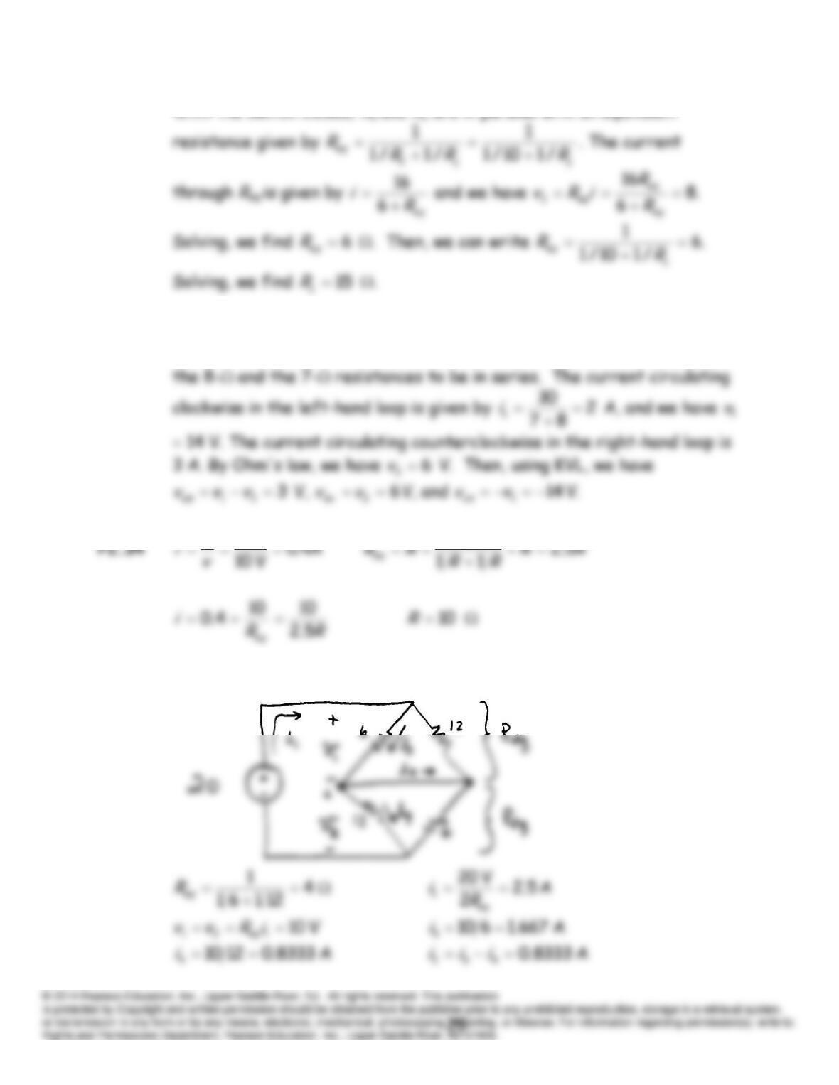
P2.33 The currents through the 3- resistance and the 4- resistance are
zero, because they are series with an open circuit. Thus, we can consider
W 4
P
1
P2.35*
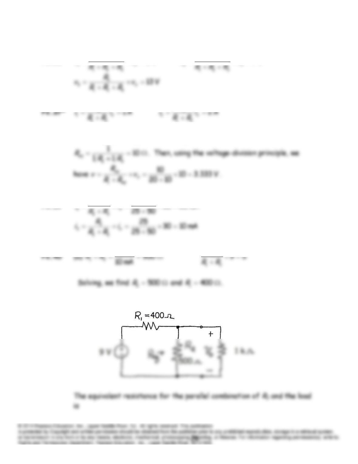
P2.36*
V 5
1
v
R
v
V 7
2
v
R
v
R
R
P2.38* Combining
2
R
and
3
R
, we have an equivalent resistance
P2.39
mA 2030
50
3
i
R
i
V 9
2
R
(b)
1
x
P2.42 First, we combine the 60 and 20 resistances in parallel yielding an
equivalent resistance of 15 , which is in parallel with
Rx
. Then, applying
x
P2.43 In a similar fashion to the solution for Problem P2.13, we can write the
following expression for the resistance seen by the 16-V source.
1
2
R
k
P2.44*
mV 50mA 1.0
w
Rv
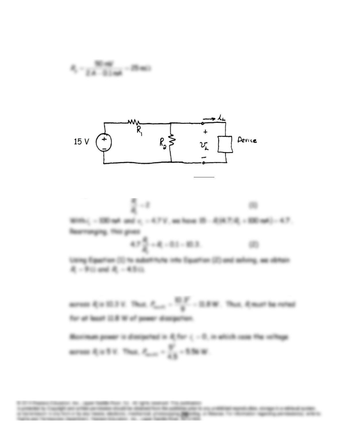
P2.45 The circuit diagram is:
With
0
L
i
and
V 5
L
v
, we must have
V 515
21
2
RR
R
. Rearranging,
this gives
mA 100
L
i
Maximum power is dissipated in
1
R
for
mA 100
L
i
, for which the voltage
1
R
1
R
0
L
i
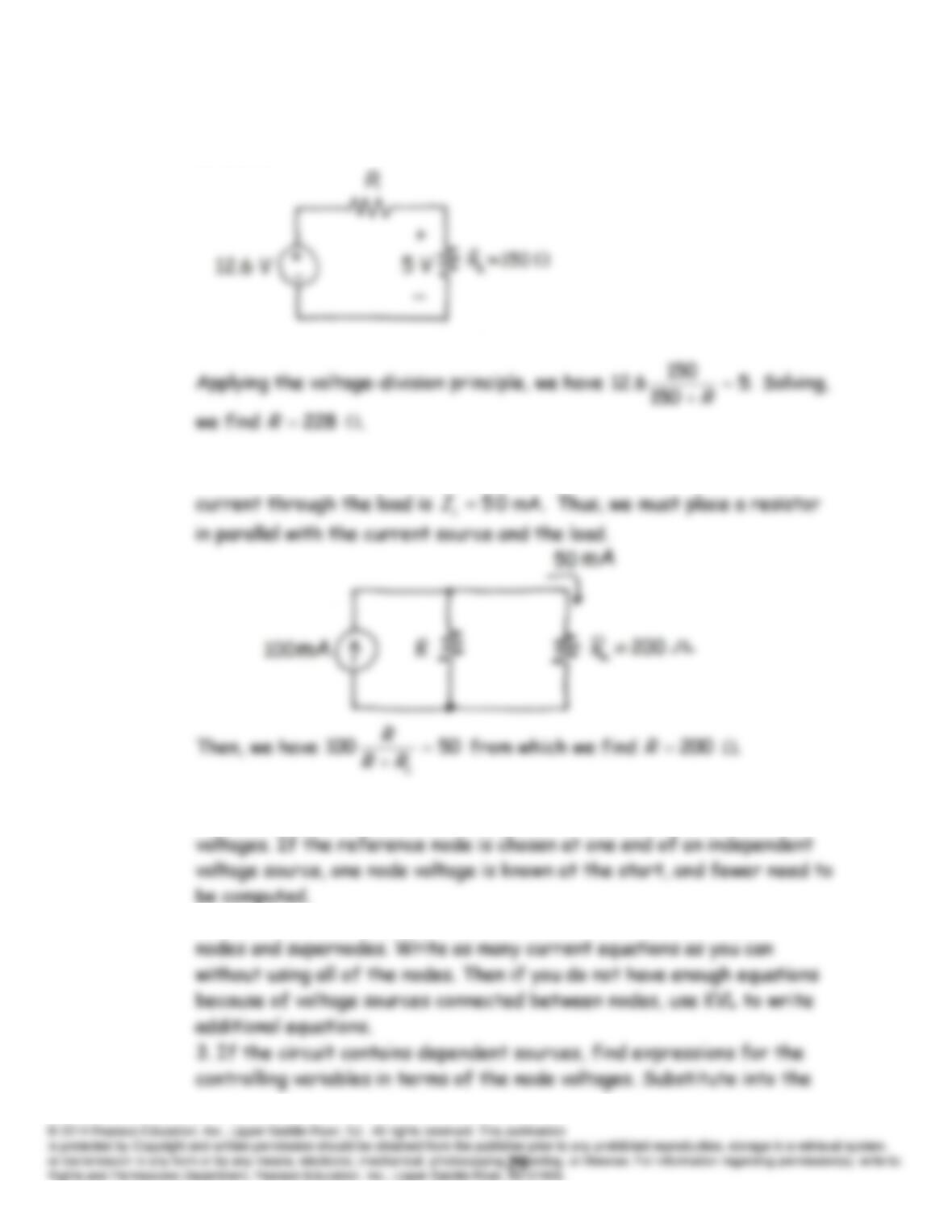
P2.46 We need to place a resistor in series with the load and the voltage source
as shown:
P2.47 We have
.20010500 223
LLL IRIP
Solving, we find that the
P2.48. 1. Select a reference node and assign variables for the unknown node
2. Write network equations. First, use KCL to write current equations for
P2.49* At node 1 we have:
1
1020
211
vvv
105
In standard form, the equations become
Solving, we find
V 29.14
1
v
and
V 43.11
2
v
.
P2.50 Writing KCL equations, we have
31
211
vv
vvv
In standard form, we have:
004545.02.03455.0 321
vvv
The MATLAB commands needed to solve are:
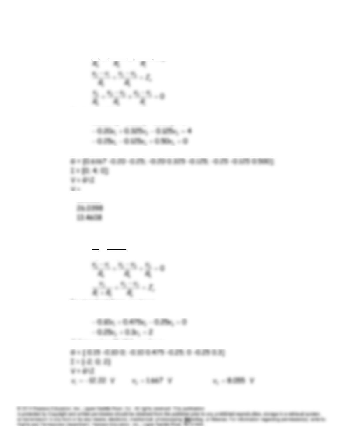
P2.51 Writing KCL equations at nodes 1, 2, and 3, we have
0
31
21
1
vv
vv
v
In standard form, we have:
025.020.06167.0 321
vvv
Using Matlab, we have
V =
13.9016
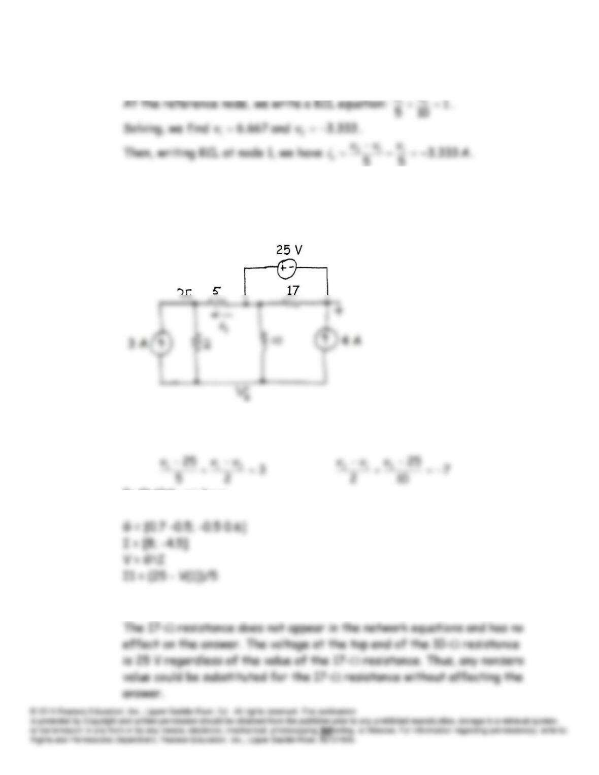
P2.52 Writing KCL equations at nodes 1, 2, and 3, we have
0
4
21
3
1
s
I
R
vv
R
v
In standard form, we have:
210.015.0 21
vv
23.025.0 32
Solving using Matlab, we have
P2.53* Writing a KVL equation, we have
10
21
vv
.
P2.54 To minimize the number of unknowns, we select the reference node at
one end of the voltage source. Then, we define the node voltages and
write a KCL equation at each node.
In Matlab, we have
Then, we have
A 2
1
i
.
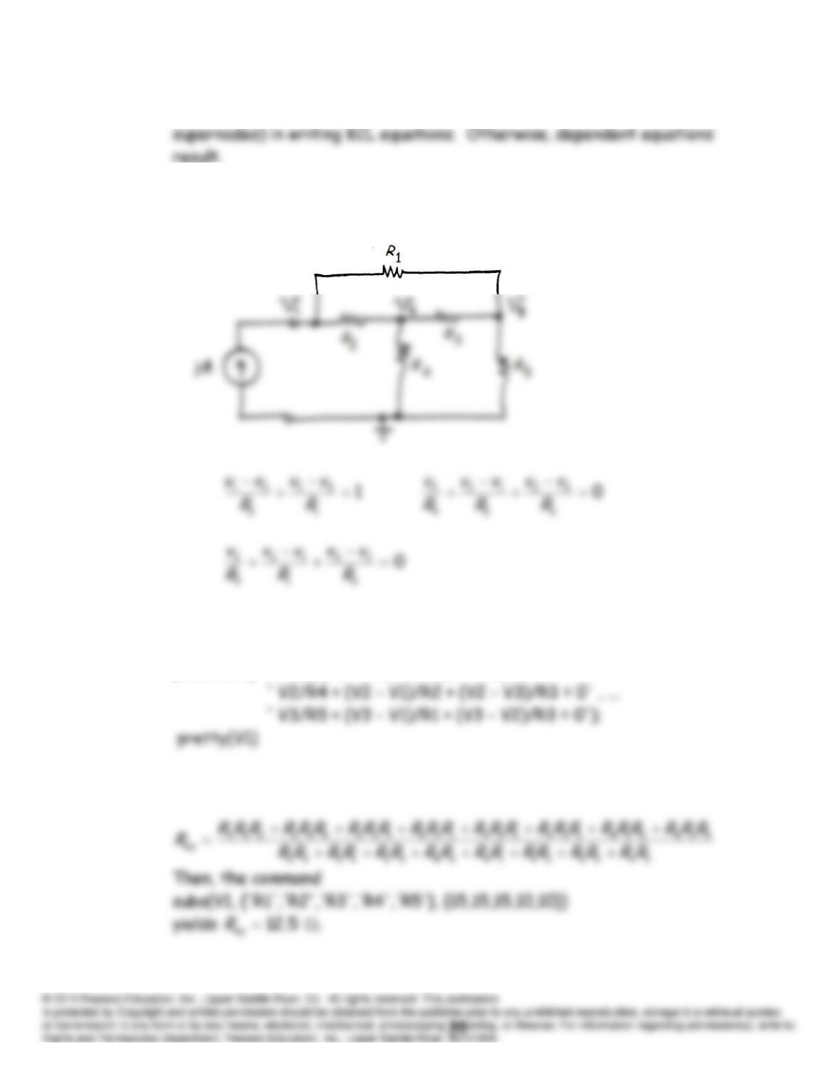
P2.55 We must not use all of the nodes (including those that are inside
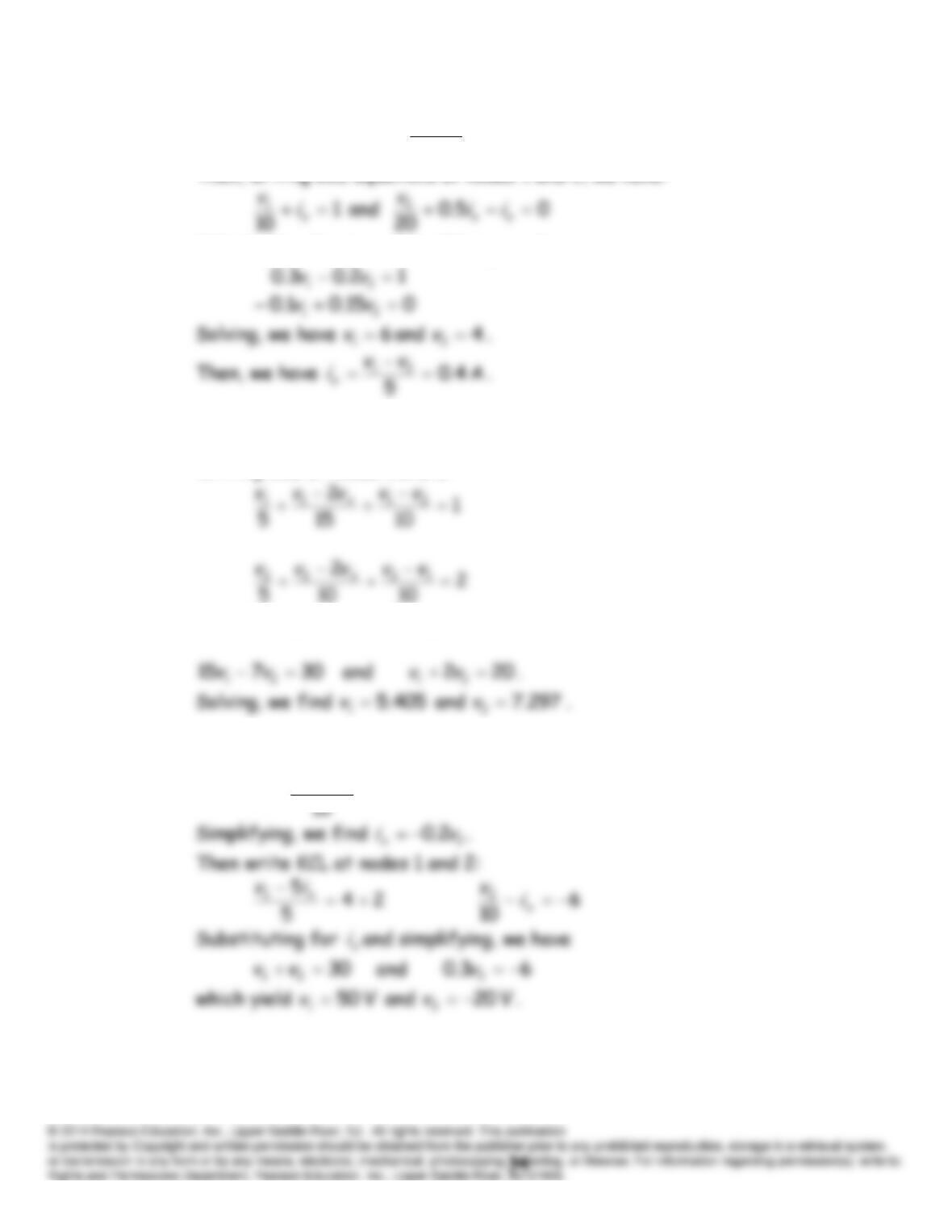
P2.56 The circuit with a 1-A source connected is:
In Matlab, we use the commands
[V1,V2,V3] = solve(‘(V1 – V2)/R2 + (V1 – V3)/R1 = 1’ , …
After some clean up, this produces
P2.57* First, we can write:
5
21
vv
ix
.
Then, writing KCL equations at nodes 1 and 2, we have:
Substituting for
x
i
and simplifying, we have
P2.58*
12
vvv x
Writing KCL at nodes 1 and 2:
Substituting and simplifying, we have
P2.59 First, we can write:
52
vi
ix
x
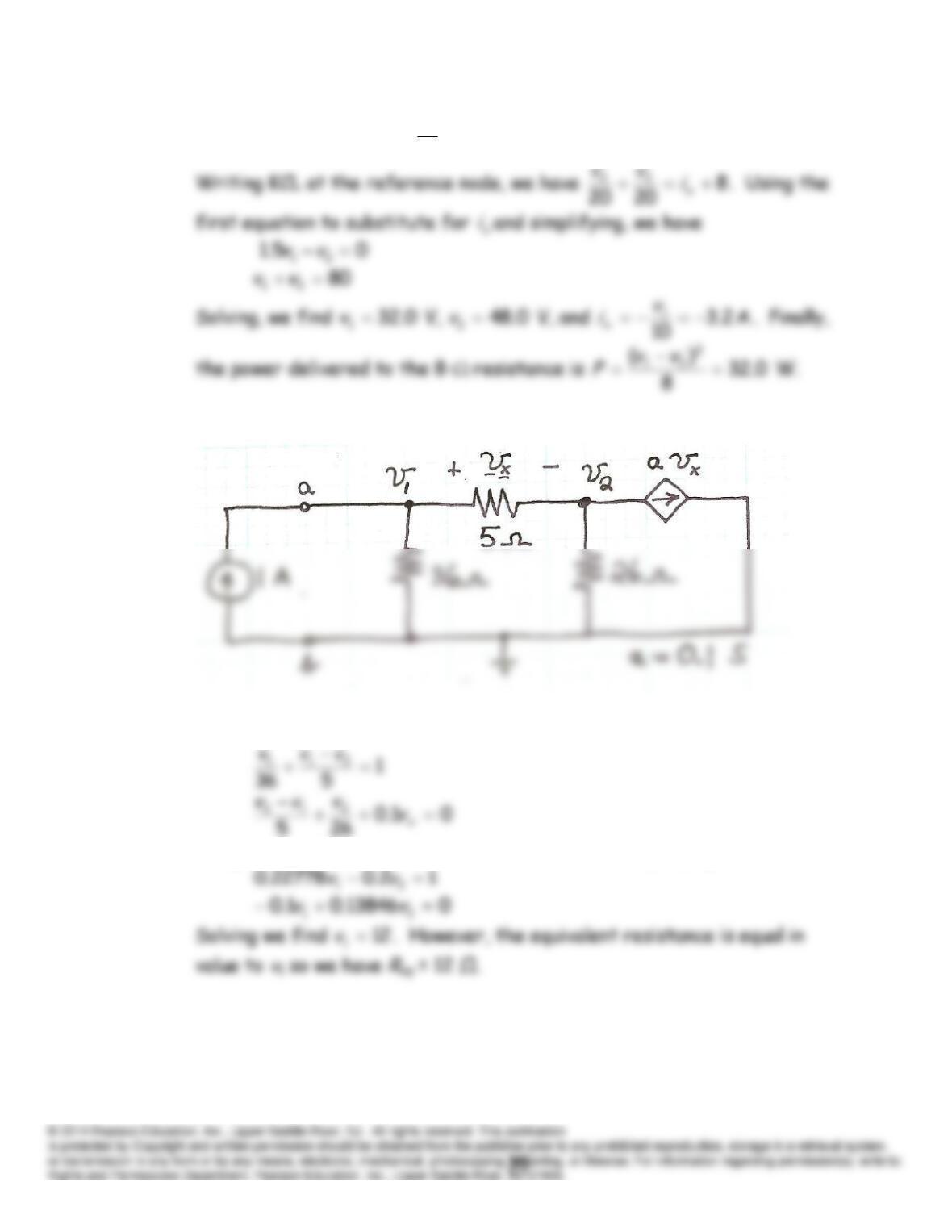
P2.60 First, we can write
10
1
v
ix
. Then writing KVL, we have
05 21
viv x
.
P2.61 The circuit with a 1-A current source connected is:
21
vvv x
Using the first equation to substitute for
vx
and simplifying, we have
P2.62 The circuit with a 1-A current source connected is
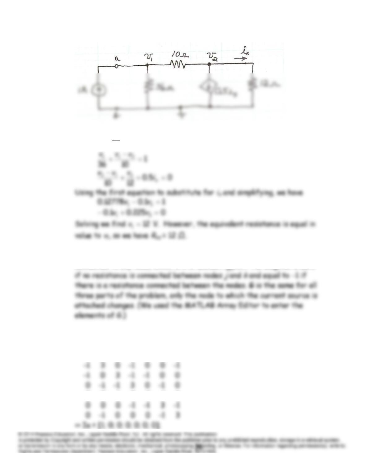
12
2
v
ix
P2.63 Elements on the diagonal of G equal the sum of the conductances
connected to any node, which is 3 S. Element
gjk
off the diagonal is zero
>> G
G =
3 -1 -1 0 0 0 0
0 0 -1 0 3 -1 0
>> Ib = [0; 1; 0; 0; 0; 0; 0];
Ra =
0.5833
0.7500
P2.64 First, we enter the node voltage equations into the solve command and
define the unknowns to be V1, V2 and Vout. Then, we use the pretty
command to print the answer for Vout:
SV = solve(‘(V1 – Vin)/(2*R1) + (V1 – Vout)/R1 + (V1 – V2)/R1 = 0′ , …
P2.65 We write equations in which voltages are in volts, resistances are in k,
and currents are in mA.
Then, using Matlab we have:
G = [-1/4 (1/2 + 1/3 + 1/4) -1/3 0; …
V =
20.7317
P2.66. 1. If necessary, redraw the network without crossing conductors or
elements. Then, define the mesh currents flowing around each of the
2. Write network equations, stopping after the number of equations is
equal to the number of mesh currents. First, use KVL to write voltage
3. If the circuit contains dependent sources, find expressions for the
4. Put the equations into standard form. Solve for the mesh currents by
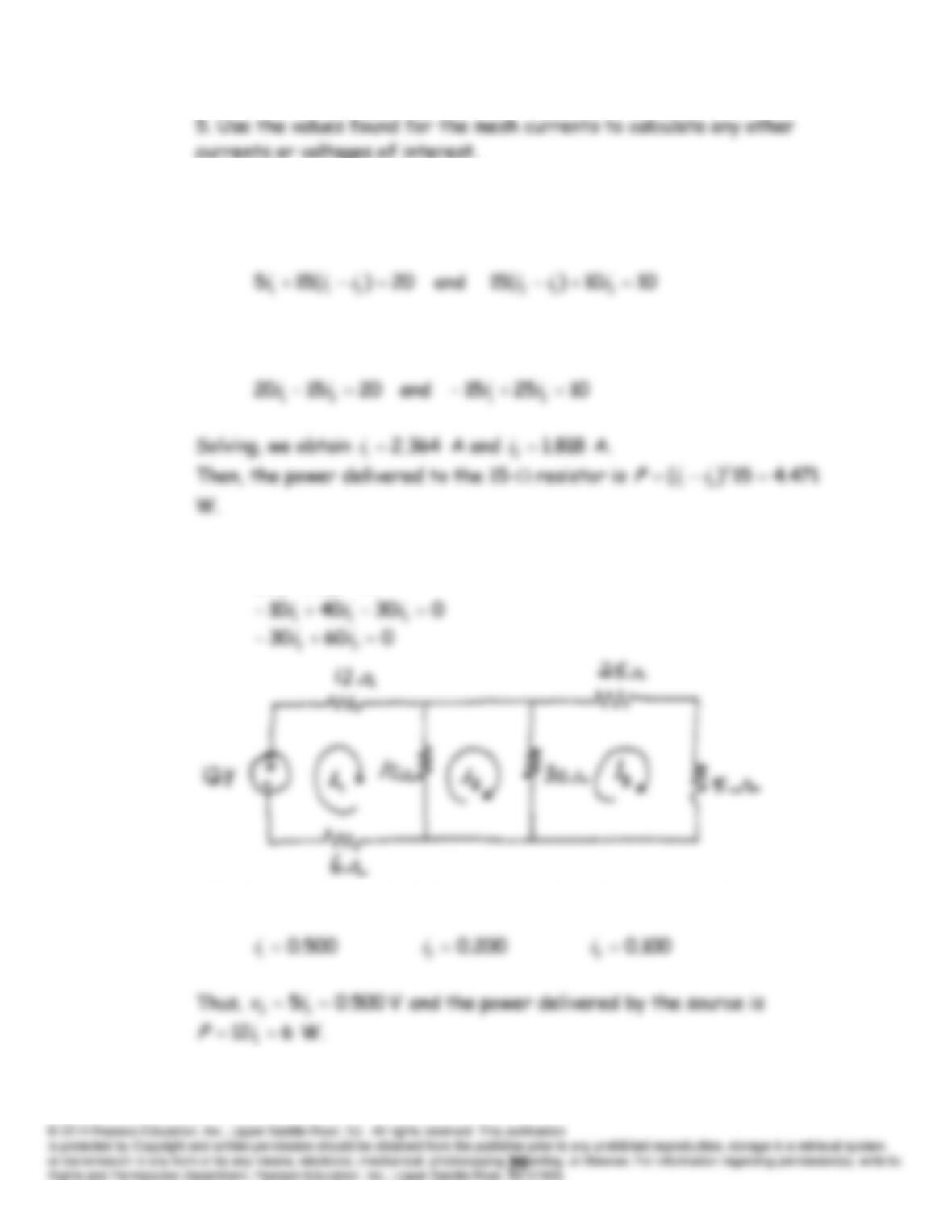
P2.67* Writing KVL equations around each mesh, we have
Putting the equations into standard from we have
P2.68* Writing and simplifying the mesh-current equations, we have:
121028 21
ii
Solving, we obtain
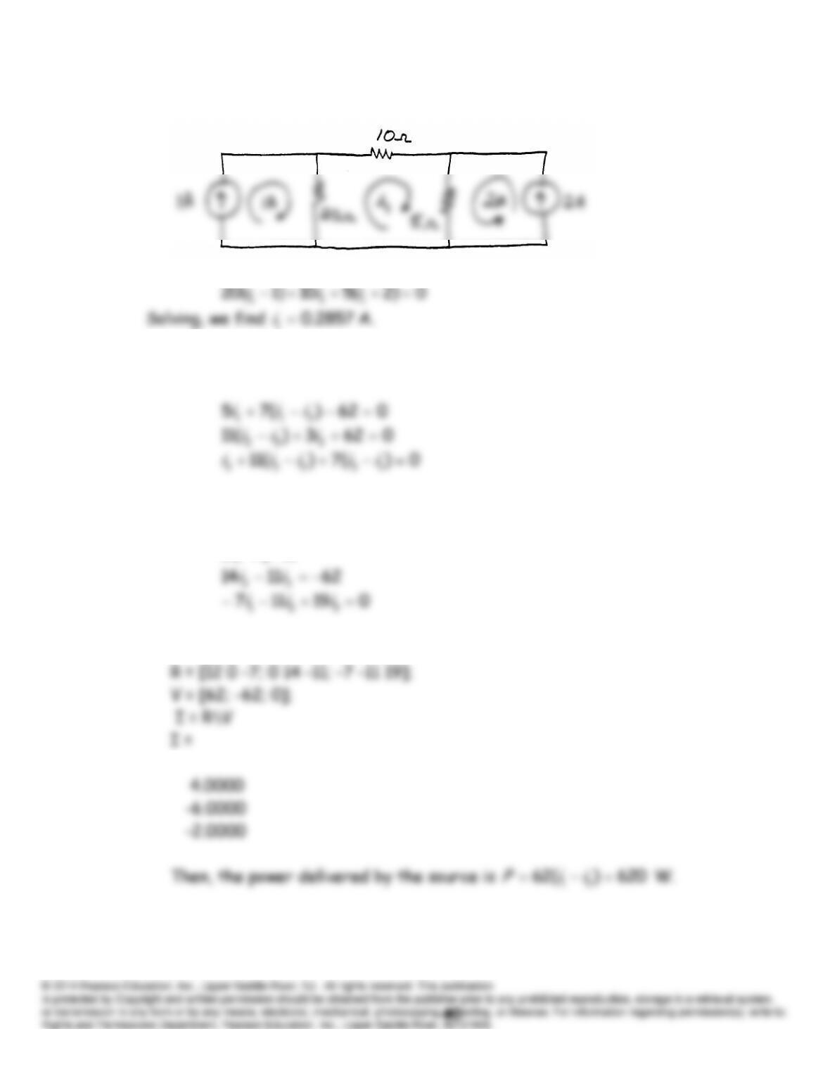
P2.69* Because of the current sources, two of the mesh currents are known.
Writing a KVL equation around the middle loop we have
P2.70 Writing KVL equations around each mesh, we have
Putting the equations into standard from, we have
62712 31
ii
Using Matlab to solve, we have
P2.71 Writing and simplifying the mesh equations, we obtain: