Problems 16–39
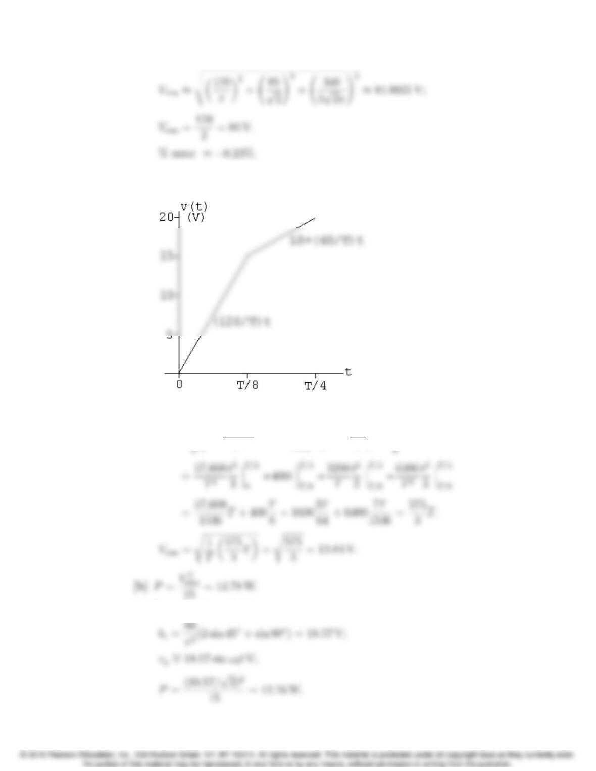
P 16.41 [a] From Problem 16.14,
The area under v2:
A=4“ZT/8
0
14,400
T2t2dt +ZT/4
T/8✓10 + 40t
T◆2
dt#
[c] From Problem 16.14,
16–40 CHAPTER 16. Fourier Series
P 16.42 [a] Half-wave symmetry av=0,a
k=bk=0,even k:
ak=4
TZT/4
0
4Im
Ttcos kω0t dt =16Im
T2ZT/4
0
tcos kω0t dt
[b] ak−jbk=2Im
πk(“sin kπ
2!−2
πk#−“j2
πksin kπ
2!#);
[c] Ig=v
u
u
t
1
X
n=1,3,5,… A2
n
2!
Problems 16–41
P 16.43 Figure P16.43(b): ta=0.2s;tb=0.6s.
v= 50t, 0≤t≤0.2;
Figure P16.43(c): ta=tb=0.4s
v(t)=25t, 0≤t≤0.4;
16–42 CHAPTER 16. Fourier Series
Figure P16.43(d): ta=tb= 1.
P 16.44 Co=Av=VmT
2·1
T=Vm
2.
P 16.45 [a] Vrms =s1
TZT
0
v2dt =s1
TZT
0✓Vm
T◆2
t2dt
T
[b] From the solution to Problem 16.44
Problems 16–43
c2=j120
4π=j30
π;c6=j120
12π=j10
π;
[c] P=(68.58)2
10 = 470.32 W;
P 16.46 Cn=1
TZT/4
0
Vmejnωotdt =Vm
T“ejnωot
−jnωo
T/4
0#
or
Co=Vm
2πlim
n!0“sin(nπ/2)
n−j1−cos(nπ/2)
n#
P 16.47 [a] Co=av=(1/2)(T/2)Vm
T=Vm
4;
[b] Co=54
4= 13.5 V;
[c]
Vo
Problems 16–45
Vo
H(j0) = 0;
Therefore,
H1=0.8/0;H1=0.8/0;
The output voltage coefficients:
C0= 0;
C2=0.2287/3.81V;
[d] Vrms ∼
=v
u
u
tC2
o+2
4
X
n=1
|Cn|2∼
=v
u
u
t2
4
X
n=1
|Cn|2
16–46 CHAPTER 16. Fourier Series
P 16.48 [a] Vrms =s1
TZT/2
0✓2Vm
Tt◆2
dt
[b] From the solution to Problem 16.47
C0= 13.5; |C3|=2.93;
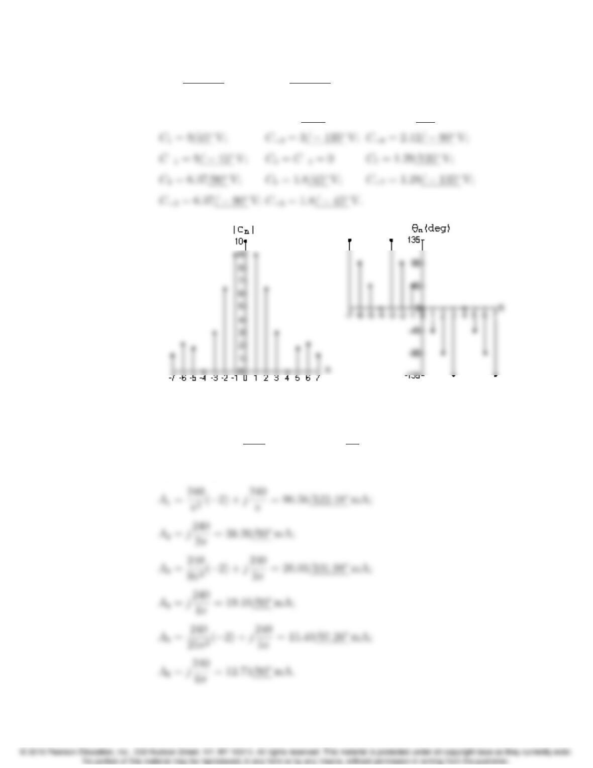
P 16.49 [a] From Example 16.3 we have:
Problems 16–47
[b] Cn=an−jbn
2,C
n=an+jbn
2=C⇤
n.
C0=av= 10 V; C3=3
/135V; C6=2.12/90V;
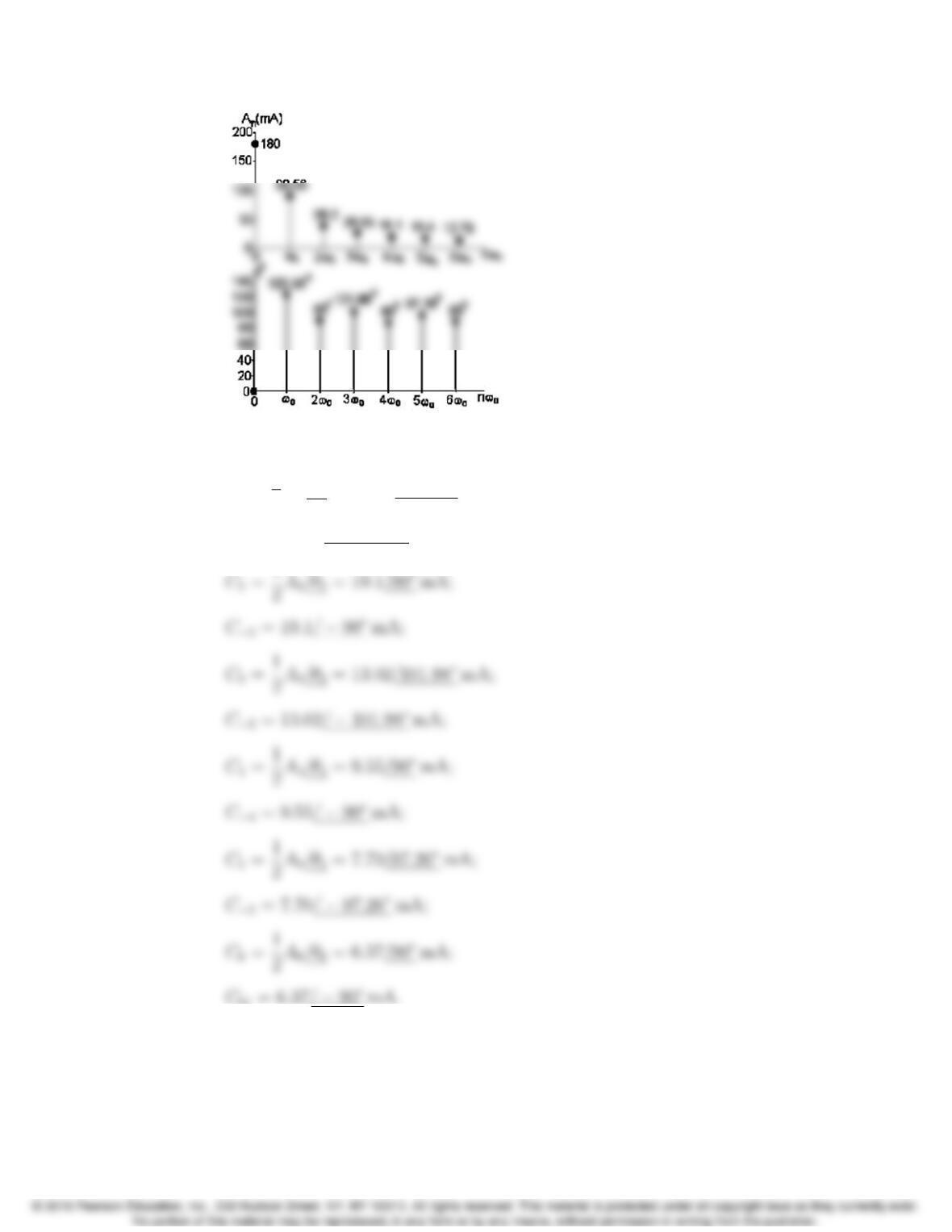
P 16.50 [a] From the solution to Problem 16.33 we have
Ak=ak−jbk=Im
π2k2(cos kπ−1) + jIm
πk.
A0=0.75Im= 180 mA;
16–48 CHAPTER 16. Fourier Series
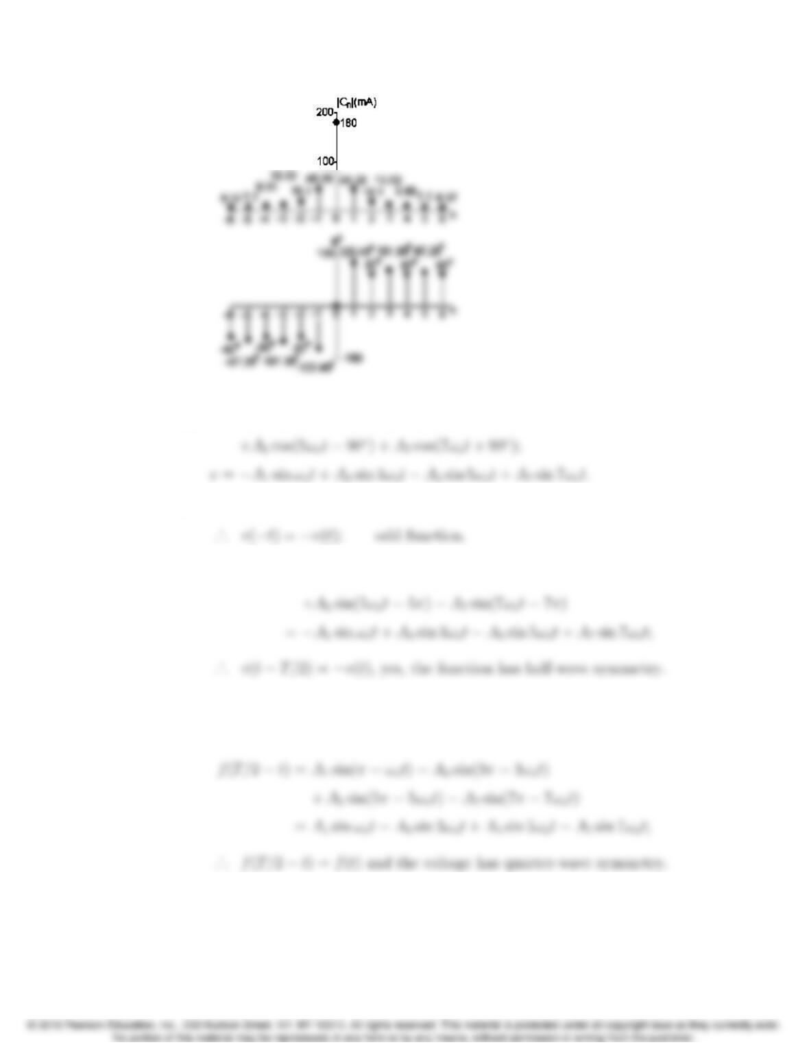
[b] C0=A0= 180 mA;
C1=1
2A1/θ1= 45.28/122.48mA;
C1= 45.28/−122.48mA;
Problems 16–49
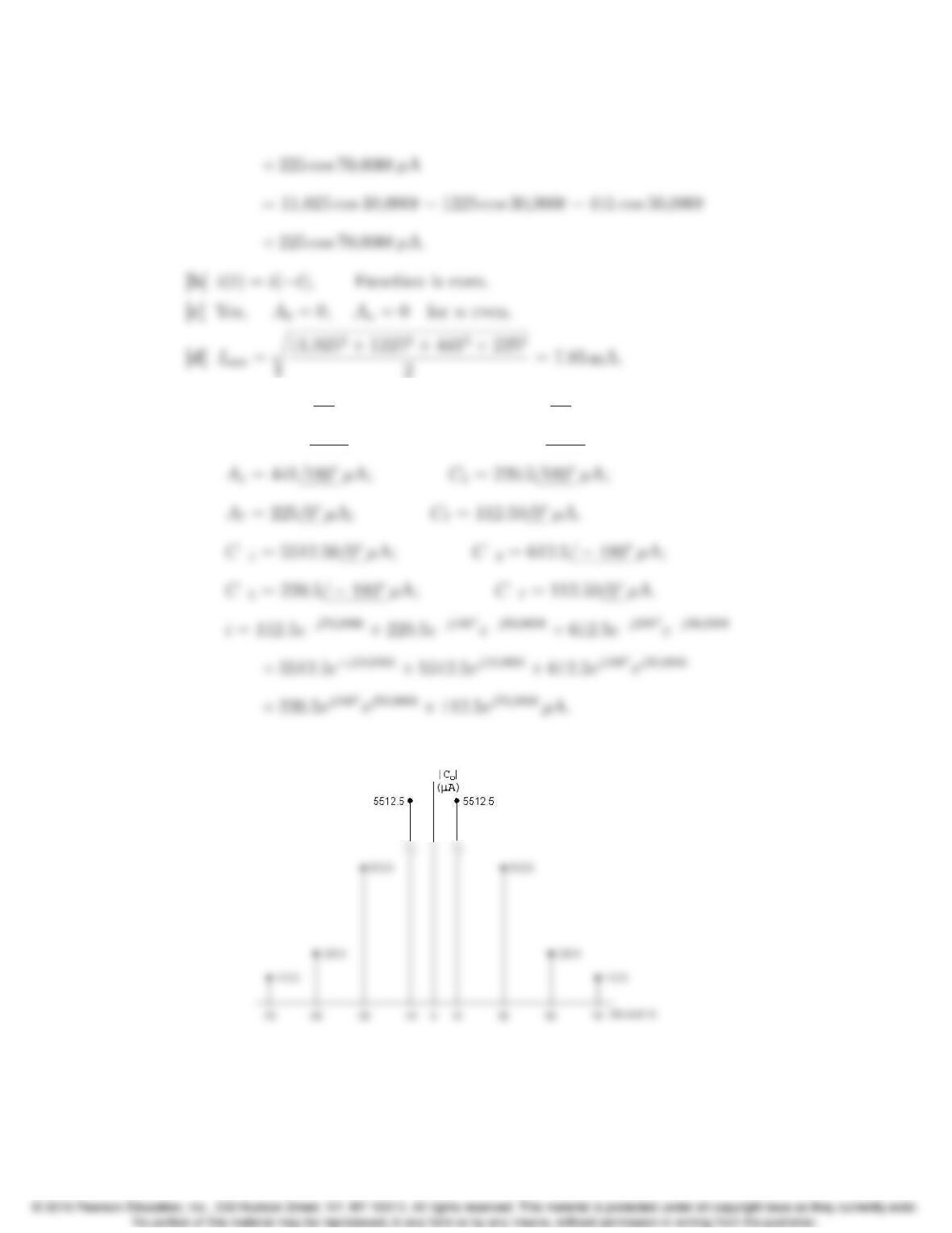
P 16.51 [a] v=A1cos(ωot−90)+A3cos(3ωot+90
)
[b] v(−t)=−A1sin ωot+A3sin 3ωot−A5sin 5ωot+A7sin 7ωot;
[c] v(t−T/2) = A1sin(ωot−π)−A3sin(3ωot−3π)
[d] Since the function is odd, with hws, we test to see if
f(T/2−t)=f(t);
16–50 CHAPTER 16. Fourier Series
P 16.52 [a] i= 11,025 cos 10,000t+ 1225 cos(30,000t−180) + 441 cos(50,000t−180)
[e] A1= 11,025/0µA; C1= 5512.50/0µA;
A3= 1225/180µA; C3= 612.5/180µA;
[f]
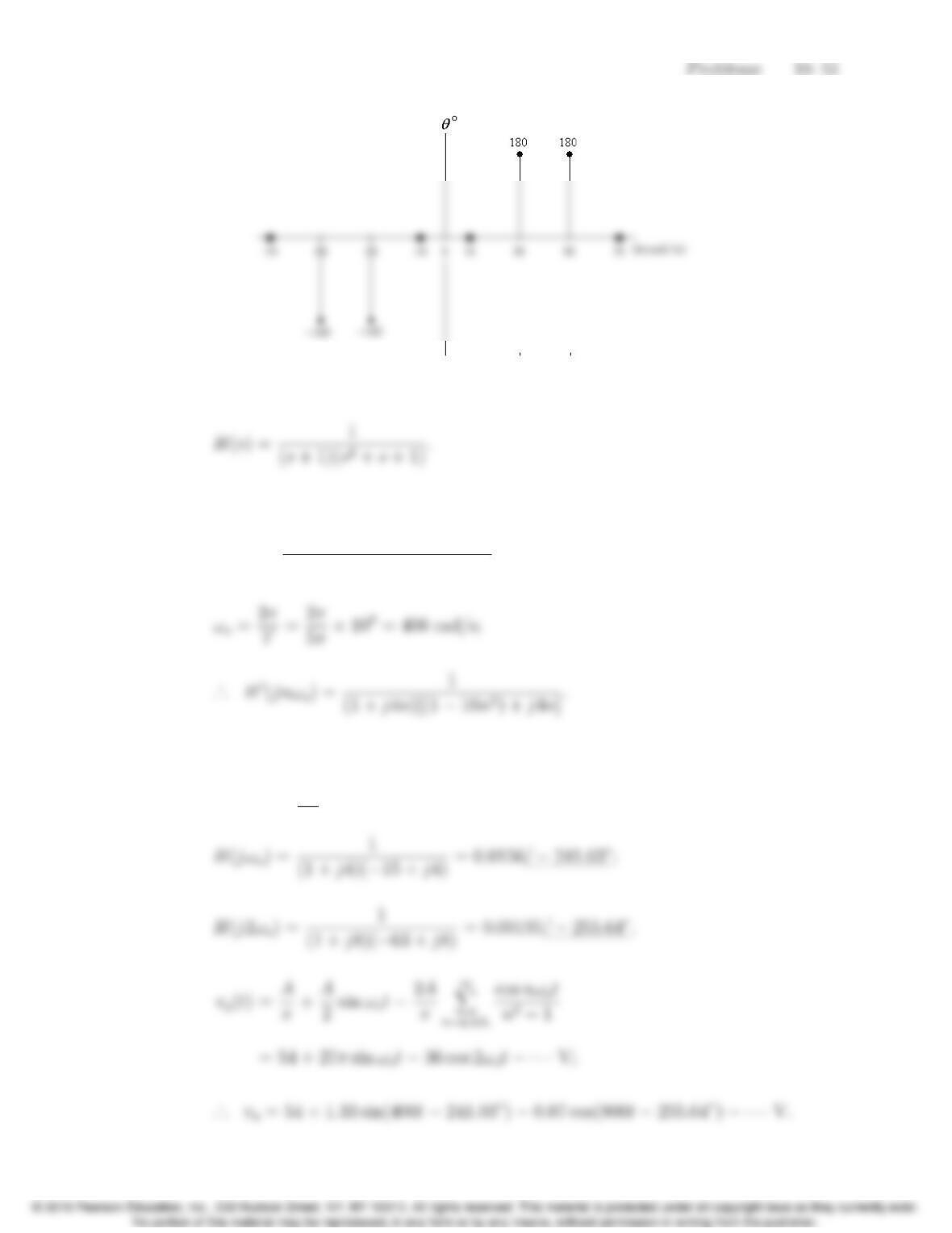
P 16.53 From Table 15.1 we have
After scaling we get
H0(s)= 106
(s+ 100)(s2+ 100s+10
4).
It follows that
H(j0) = 1/0;
16–52 CHAPTER 16. Fourier Series
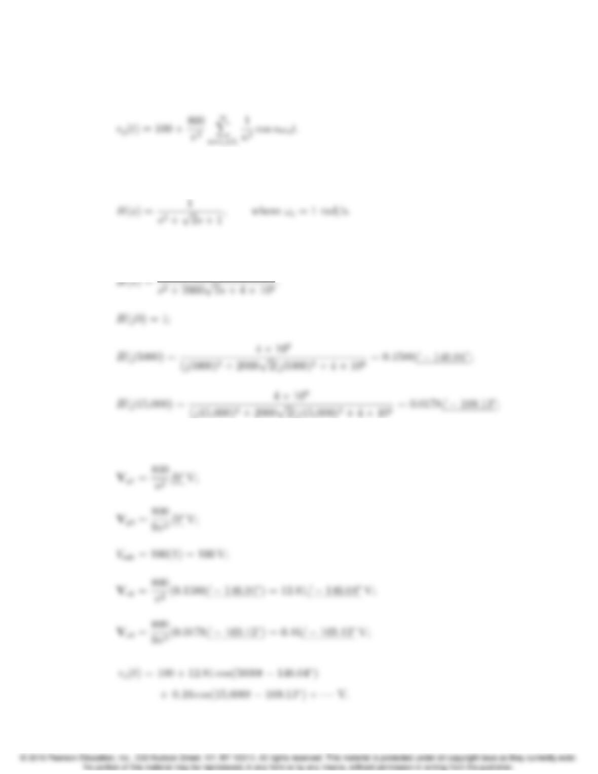
P 16.54 Using the technique outlined in Problem 16.18 we can derive the Fourier series
for vg(t). We get
The transfer function of the prototype second-order low pass Butterworth
filter is
Now frequency scale using kf= 2000 to get ωc= 2 krad/s:
Vdc = 100 V;
Problems 16–53
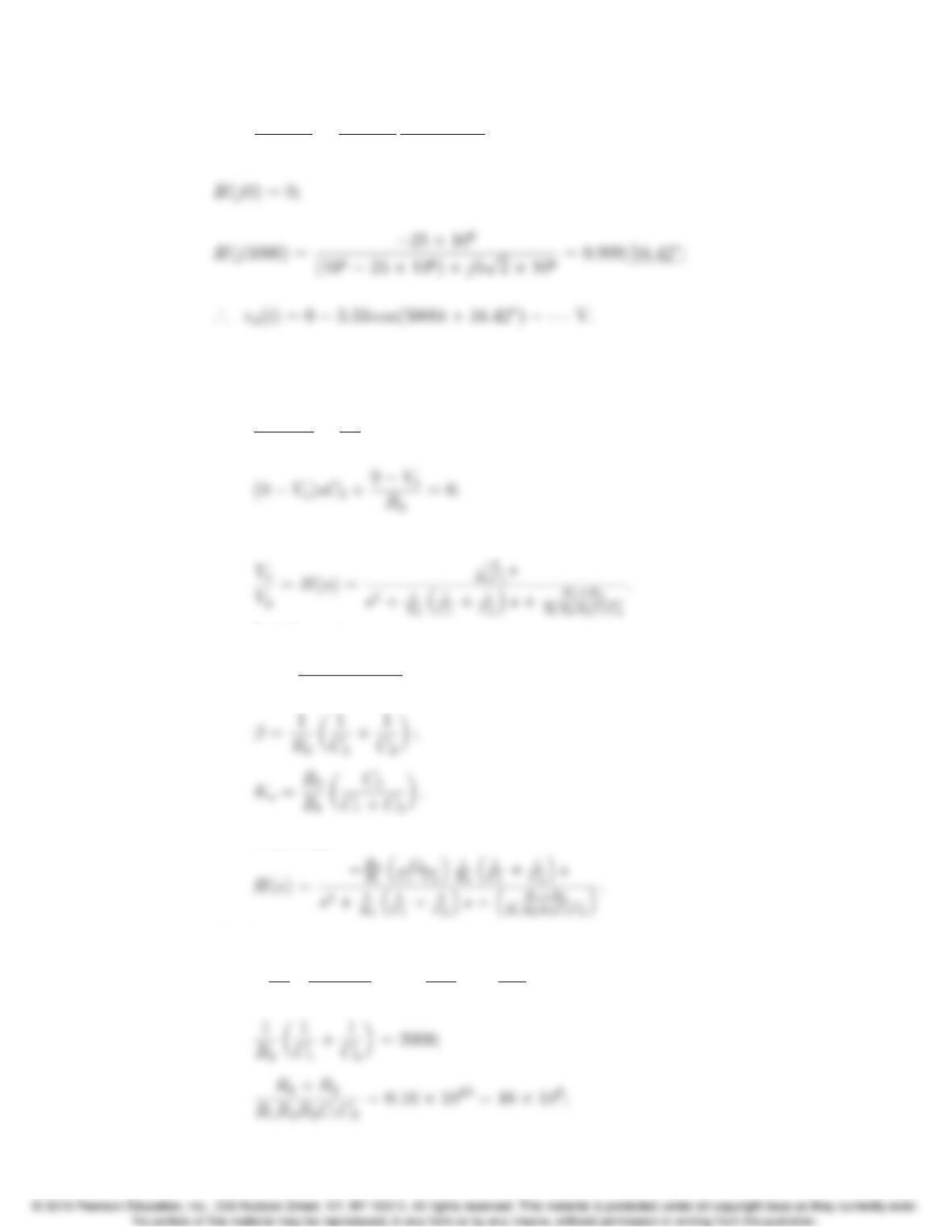
P 16.55 vg=2(2.5π)
π−4(2.5π)
π
(cos 5000t)
4−1=5−(10/3) cos 5000t−···V.
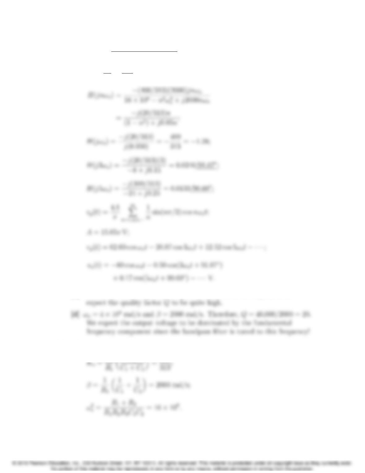
P 16.56 [a] Let Varepresent the node voltage across R2, then the node-voltage
equations are
Va−Vg
R1
+Va
R2
+VasC2+(Va−Vo)sC1= 0;
Solving for Voin terms of Vgyields
It follows that
ω2
o=R1+R2
R1R2R3C1C2
Note that
[b] For the given values of R1,R
2,R
3,C
1, and C2we have
−R3
R1✓C2
C1+C2◆=−R3
2R1
=−400
313;
16–54 CHAPTER 16. Fourier Series
H(s)= −(400/313)(2000)s
s2+ 2000s+16×108.
ωo=2π
T=2π
50π×106=4×10⁴rad/s;
[c] The fundamental frequency component dominates the output, so we
P 16.57 [a] Using the equations derived in Problem 16.56(a),
Problems 16–55
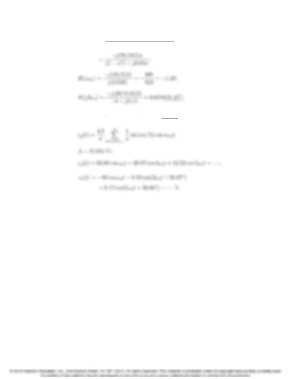
[b] H(jnωo)= −(400/313)(2000)jnωo
16 ×108−n2ω2
o+j2000nωo
H(j5ωo)=−j(100/313)
−24 + j0.25 =0.0133/90.60;