Active Filter Circuits
Assessment Problems
AP 15.1
H(s)= (R2/R1)s
s+ (1/R1C);
AP 15.2
H(s)= (1/R1C)
s+ (1/R2C)=20,000
s+ 5000.
15–1
15
15–2 CHAPTER 15. Active Filter Circuits
AP 15.3
ωc=2πfc=2π⇥104= 20,000πrad/s;
AP 15.4 For a 2nd order Butterworth high pass filter
For the circuit in Fig. 15.25
Equate the transfer functions. For C= 1F,
AP 15.5
Q=8,K =5,ω
o= 1000 rad/s,C =1µF.
For the circuit in Fig 15.26
Problems 15–3
·
Solving for R2,
AP 15.6
ωo= 1000 rad/s; Q= 4;
H(s)= s2+ (1/R2C2)
s2+“4(1 σ)
RC #s+✓1
R2C2◆
15–4 CHAPTER 15. Active Filter Circuits
Problems
P 15.1 [a] K= 10(5/20) =1.778 = R2
R1
;
[b]
P 15.2 [a] 1
RfC=2π(10,000) so RfC=1.5915 ⇥105.
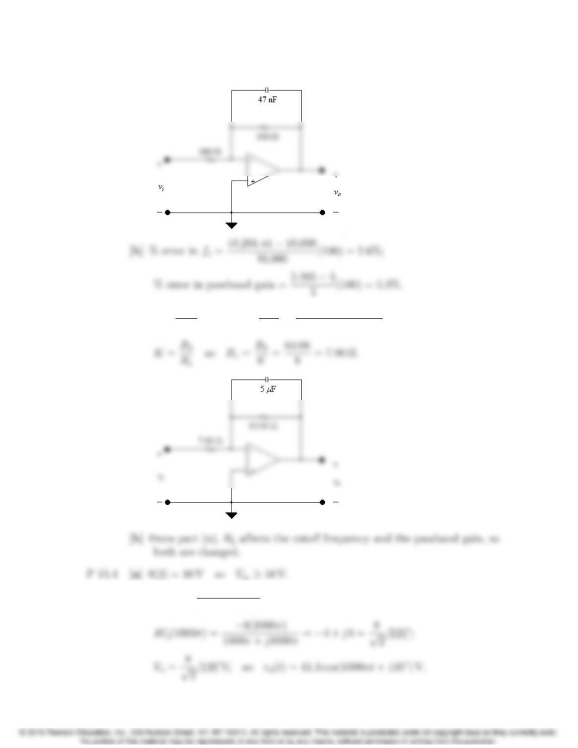
There are several possible approaches. Here, choose C= 47 nF. Then
To get a passband gain of 5 dB,
Problems 15–5
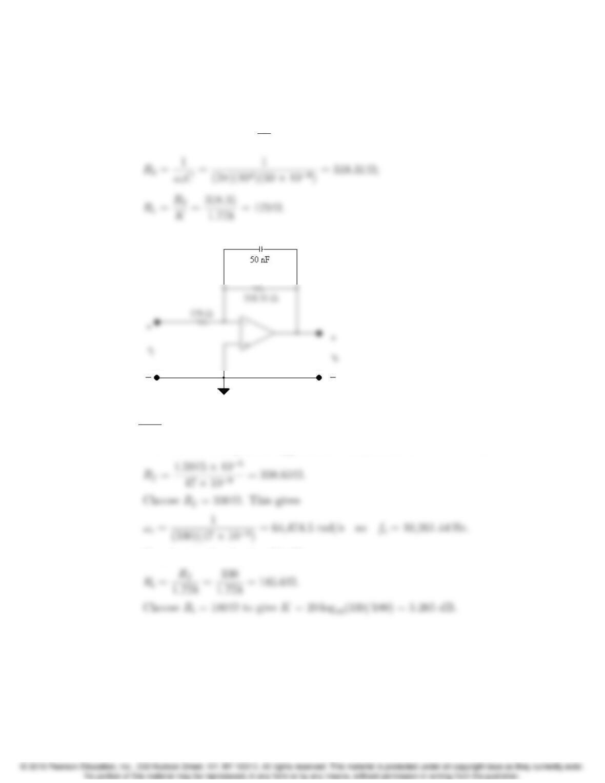
The resulting circuit is
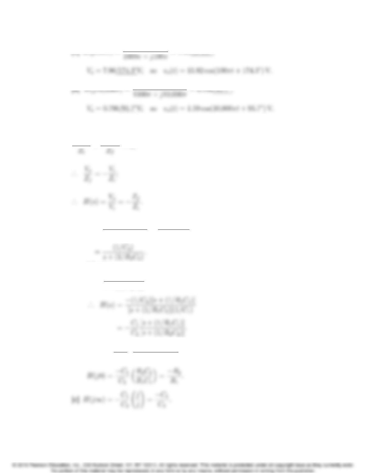
P 15.3 [a] ωc=1
R2Cso R2=1
ωcC=1
2π(500)(5 ⇥106)= 63.66 Ω;
[b] H(jω)= 8(2π)(500)
jω+2π(500).
15–6 CHAPTER 15. Active Filter Circuits
[c] H(j100π)= 8(1000π)
P 15.5 Summing the currents at the inverting input node yields
0Vi
+0Vo
= 0;
P 15.6 [a] Zf=R2(1/sC2)
[R2+ (1/sC2)] =R2
R2C2s+1
Likewise
Zi=(1/C1)
s+ (1/R1C1).
[b] H(jω)=C1
C2“jω+ (1/R1C1)
jω+ (1/R2C2)#;
Problems 15–7
[d] As ω!0 the two capacitor branches become open and the circuit reduces
to a resistive inverting amplifier having a gain of R2/R1.
P 15.7 [a] Zf=(1/C2)
s+ (1/R2C2);
jω
P 15.8 [a] R1=1
ωcC=1
(2π)(2500)(50 ⇥109)= 1273.24 Ω;
15–8 CHAPTER 15. Active Filter Circuits
[b]
P 15.9 [a] 1
R1C=2π(2500) so R1C=6.366 ⇥105.
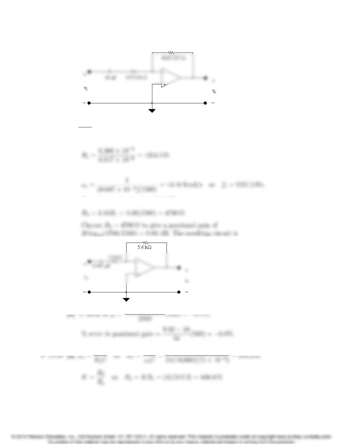
There are several possible approaches. Here, choose C=0.047 µF. Then
Choose R1= 1500 Ω. This gives
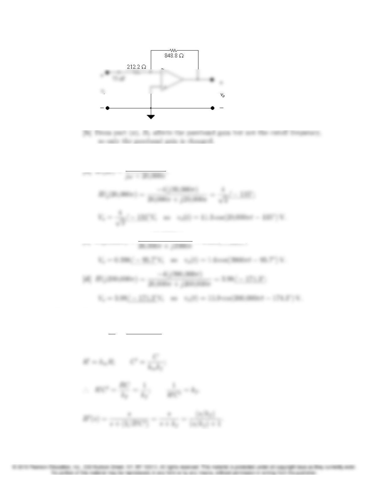
To get a passband gain of 10 dB, choose
Problems 15–9
P 15.11 [a] 4(4) = 16 V so Vcc 16 V.
[c] H(j2000π)= 4(j2000π)
P 15.12 For the RC circuit
H(s)=Vo
Vi
=s
s+ (1/RC);
15–10 CHAPTER 15. Active Filter Circuits
For the RL circuit
H(s)= s
s+(R/L);
P 15.13 For the RC circuit
H(s)=Vo
Vi
=(1/RC)
s+ (1/RC);
For the RL circuit H(s)= R/L
s+R/L so
R0=kmR;L0=km
kf
L;
Problems 15–11
P 15.14 H(s)= (R/L)s
s2+(R/L)s+ (1/LC)=βs
s2+βs+ω2
o
.
For the prototype circuit ωo= 1 and β=ωo/Q =1/Q.
For the scaled circuit
therefore the Qof the scaled circuit is the same as the Qof the unscaled
circuit. Also note β0=kfβ.
·
0(s)= ⇣kf
Q⌘s
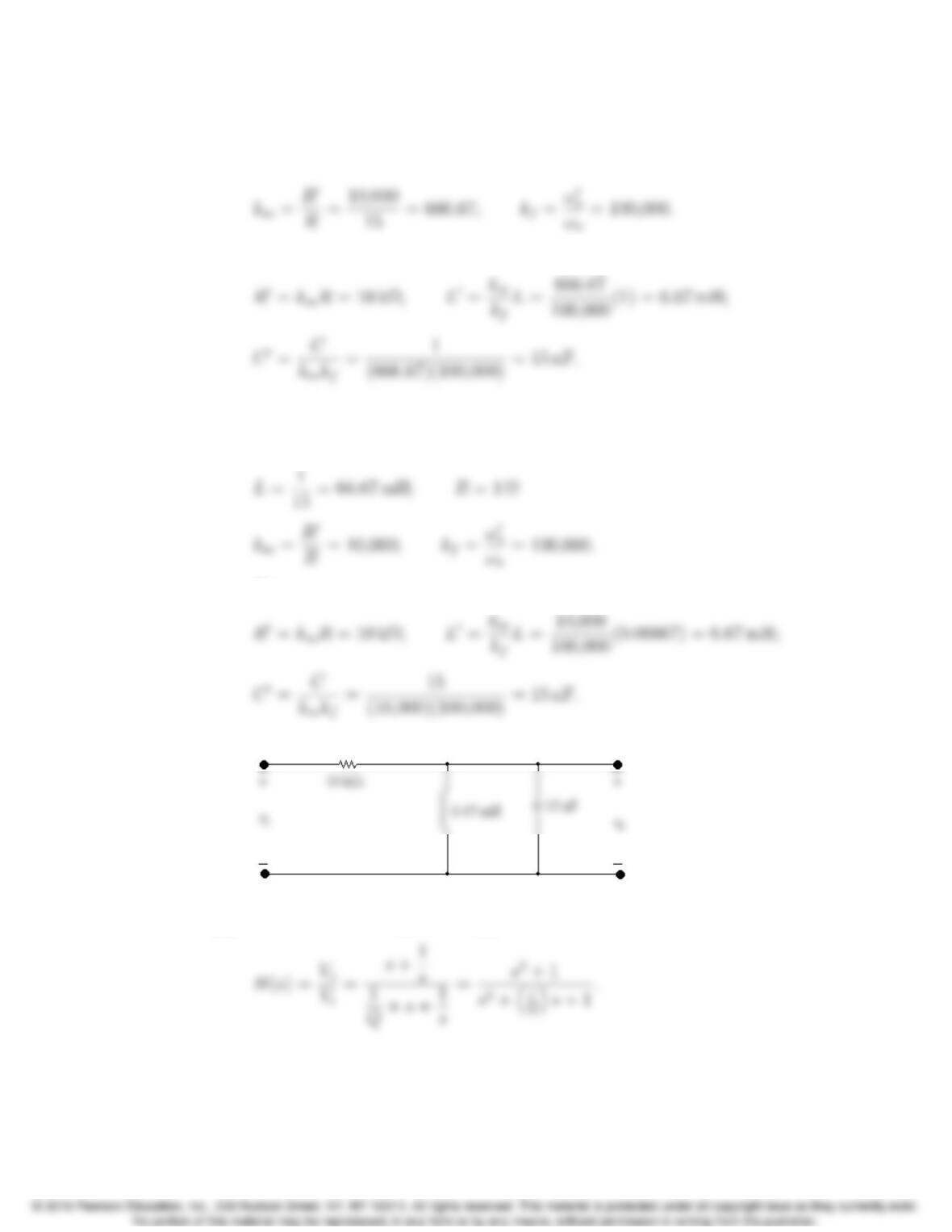
P 15.15 [a] L= 1 H; C= 1 F;
[b] kf=ω0
o
ωo
= 75,000; km=R0
R=2500
0.1= 25,000.
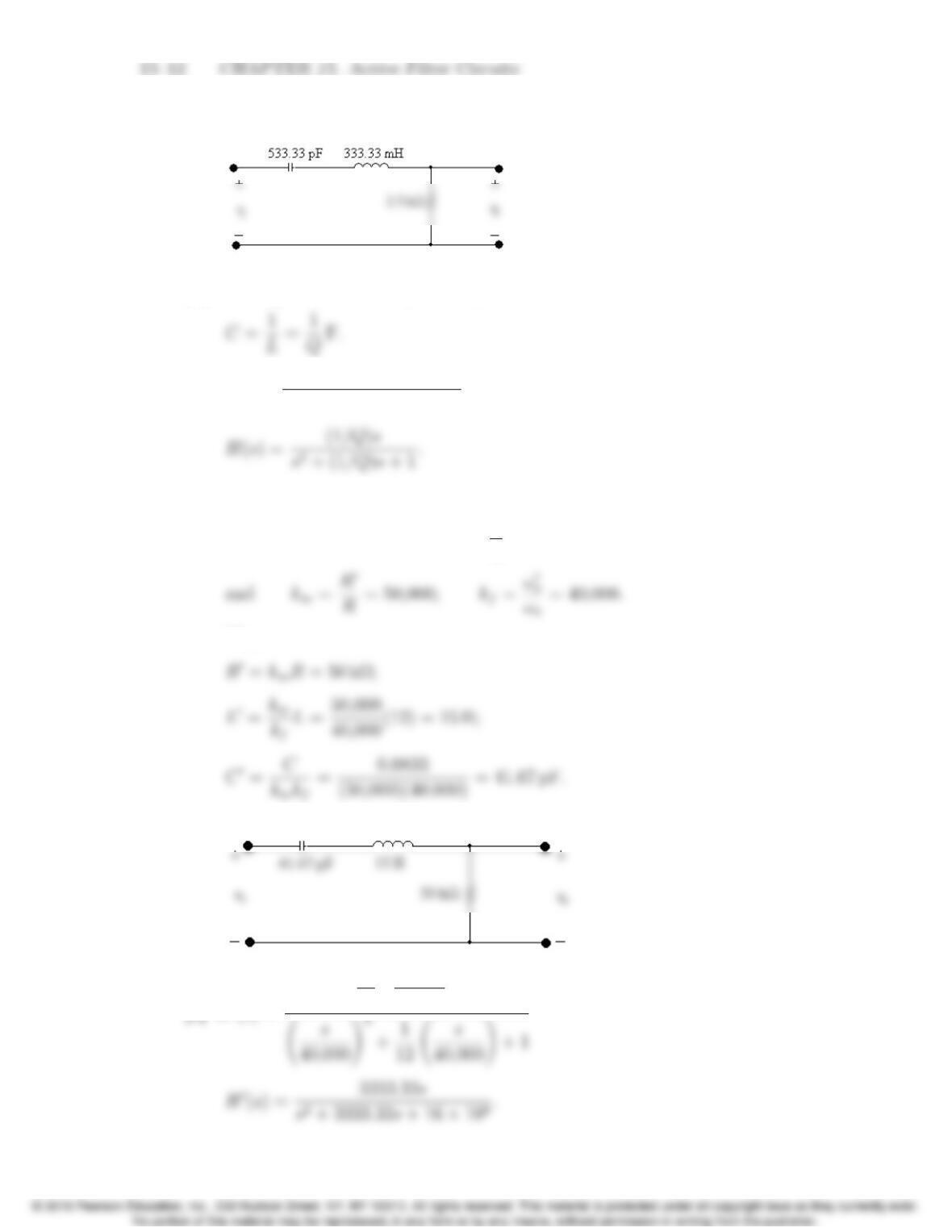
Thus,
[c]
P 15.16 [a] Since ω2
o=1/LC and ωo= 1 rad/s,
[b] H(s)= (R/L)s
s2+(R/L)s+ (1/LC);
[c] In the prototype circuit
R= 1 Ω;L= 12 H; C=1
L=0.0833 F;
Thus
[d]
[e] H0(s)=
1
12 s
40,000!
Problems 15–13
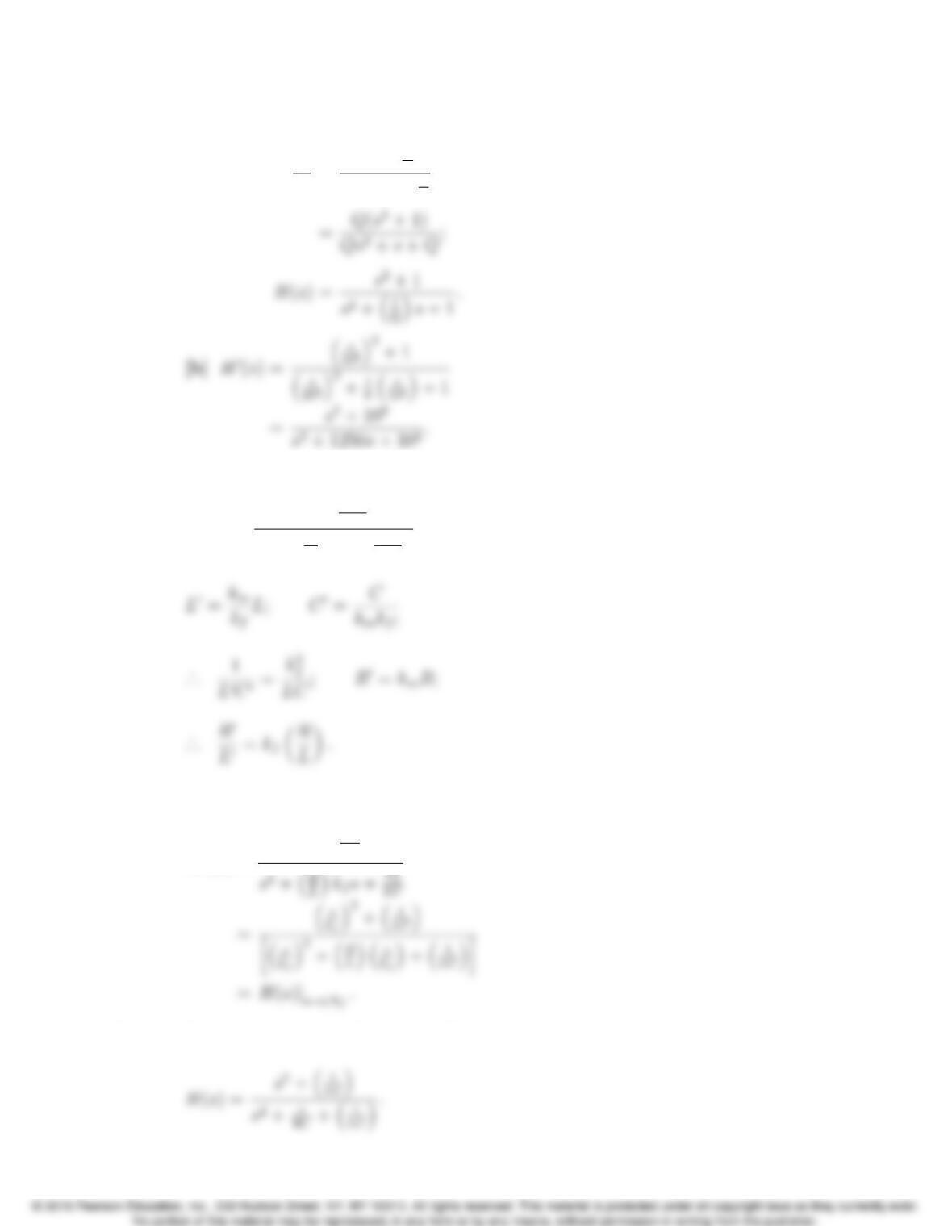
P 15.17 [a] Using the first prototype
ωo= 1 rad/s; C= 1 F; L= 1 H; R= 15 Ω.
Thus,
Using the second prototype
ωo= 1 rad/s; C= 15 F;
Thus,
[b]
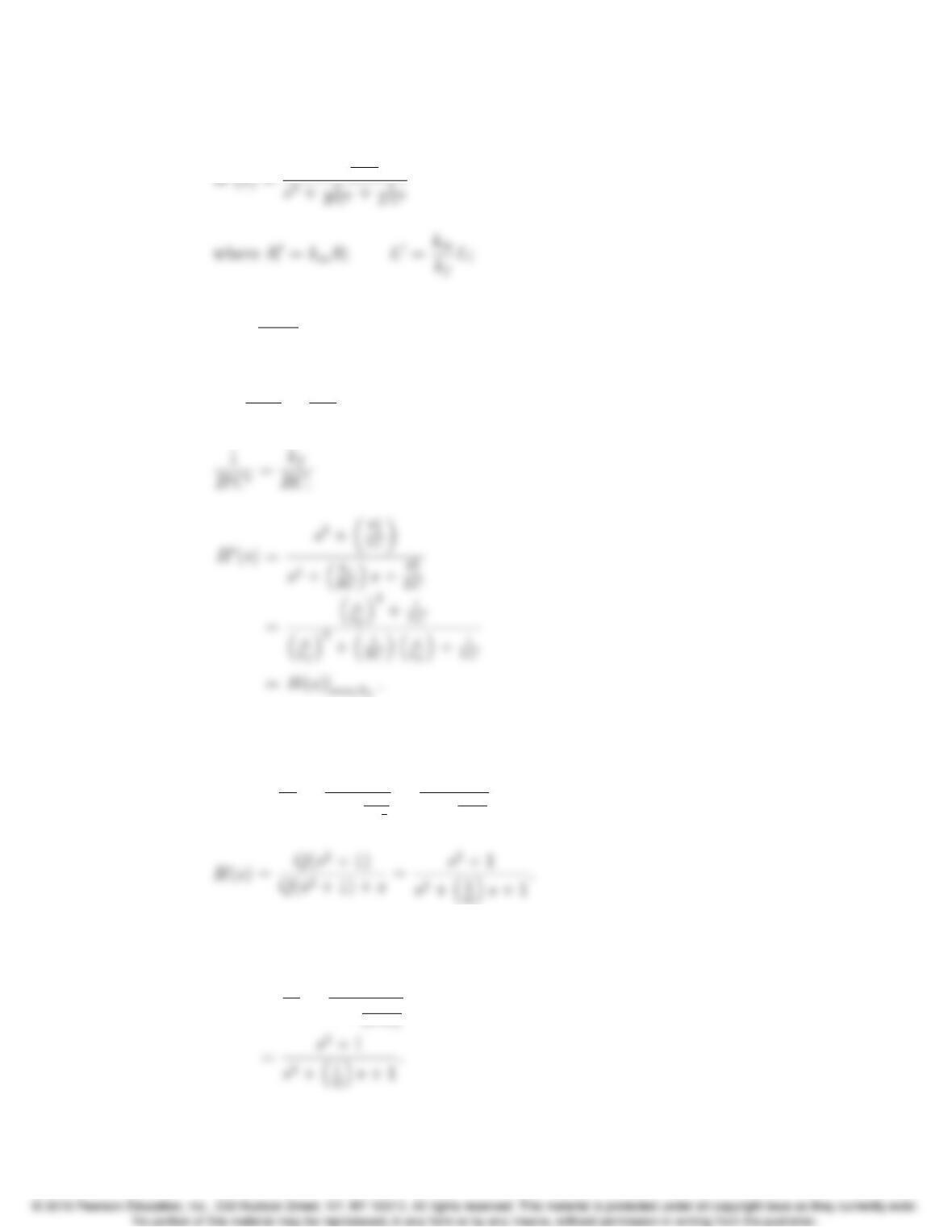
P 15.18 [a] For the circuit in Fig. P15.18(a)
15–14 CHAPTER 15. Active Filter Circuits
For the circuit in Fig. P15.18(b)
H(s)=Vo
Vi
=Qs +Q
s
1+Qs +Q
s
P 15.19 For the scaled circuit
H0(s)= s2+⇣1
L0C0⌘
s2+⇣R0
L0⌘s+⇣1
L0C0⌘;
It follows then that
H0(s)=
s2+✓k2
f
LC ◆
P 15.20 For the circuit at the bottom of Fig. 14.31
Problems 15–15
It follows that
L0C0
C0=C
kmkf
;
·
.. 1
L0C0=k2
f
LC .
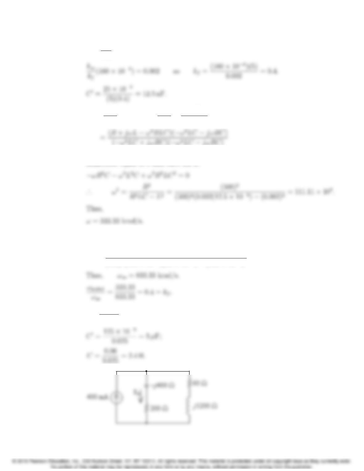
P 15.21 For prototype circuit (a):
H(s)=Vo
Vi
=Q
Q+1
s+1
s
=Q
Q+s
s2+1
;
For prototype circuit (b):
H(s)=Vo
Vi
=1
1+ (s/Q)
15–16 CHAPTER 15. Active Filter Circuits
P 15.22 [a] km=500
100 = 5;
[b] Zab =1
jωC+RkjωL=1
jωC+jωRL
R+jωL
The denominator is purely real, so set the imaginary part of the
numerator equal to 0 and solve for ω:
[c] In the original, unscaled circuit, the frequency at which the impedance Zab
is purely real is
ω2
us =(100)2
(100)2(160 ⇥106)(25 ⇥109)(160 ⇥106)2= 694.44 ⇥109.
P 15.23 [a] kf=500
20,000 =0.025;
Problems 15–17
P 15.24 From the solution to Problem 14.30, ωo= 100 krad/s and β= 12.5 krad/s.
Compute the two scale factors:
kf=ω0
o
ωo
=2π(200 ⇥103)
100 ⇥103=4π;
Thus,
π= 2546.45 ΩL0=km
kf
4π(10 ⇥103) = 253.3µH.
Calculate the cutofffrequencies:
P 15.25 From the solution to Problem 14.41, ωo= 106rad/s and β=2π(10.61) krad/s.
Calculate the scale factors:
Thus,
15–18 CHAPTER 15. Active Filter Circuits
Calculate the bandwidth:
To check, calculate the quality factor:
P 15.26 [a] From Eq 15.1 we have
H(s)=Kωc
s+ωc
where K=R2
R1
,ω
c=1
R2C;
P 15.27 [a] From Eq. 15.4
H(s)= Ks
where K=R2
and
Problems 15–19
1C0.
By hypothesis
P 15.28 [a] Hhp =s
s+1;kf=ω0
o
ω=1000(2π)
1= 2000π;
0
15–20 CHAPTER 15. Active Filter Circuits
[b] H0(s)= s
s+ 2000π·10,000π
s+10,000π
[c] ωo=pωc1ωc1=q(2000π)(10,000π) = 1000πp20 rad/s;
[e]
P 15.29 [a] For the high-pass section:
kf=ω0
o
ω=4000(2π)
1= 8000π;
For the low-pass section:
kf=ω0
o
ω=400(2π)
1== 800π;