12–18 CHAPTER 12. Introduction to the Laplace Transform
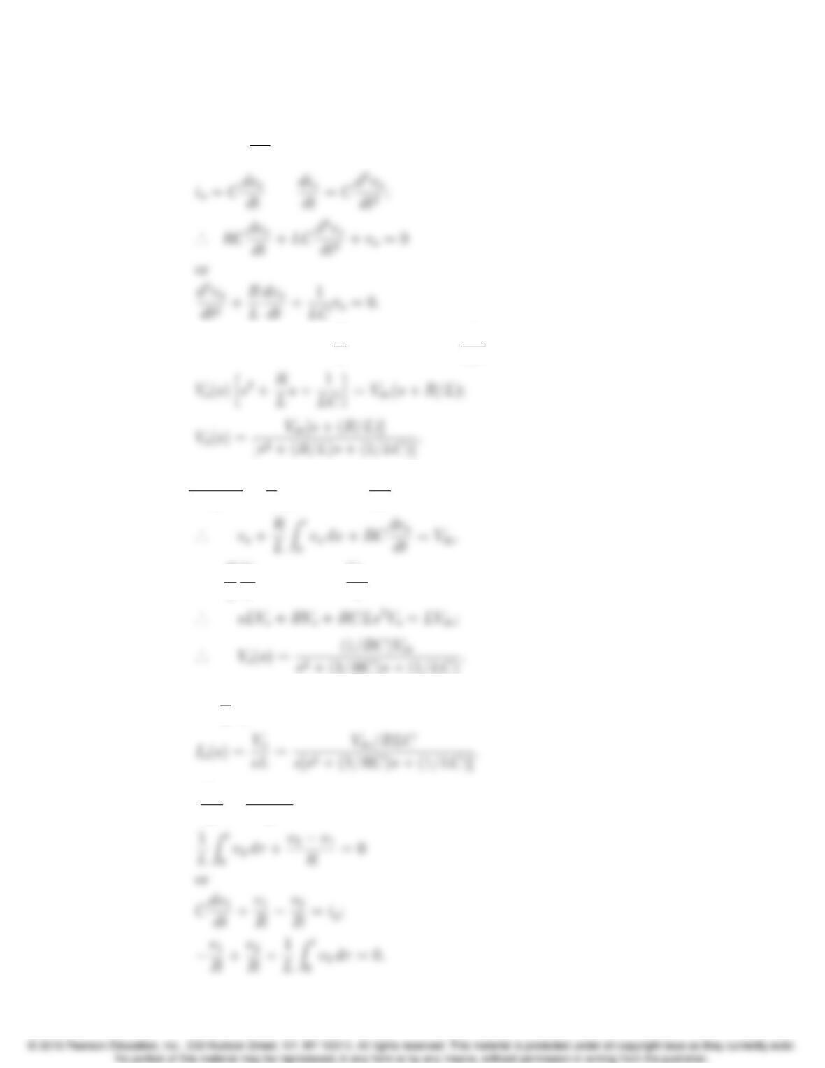
P 12.29 [a] For t≥0+:
Rio+Ldio
dt +vo= 0;
[b] s2Vo(s)−sVdc −0+R
L[sVo(s)−Vdc]+ 1
LC Vo(s)=0;
P 12.30 [a] vo−Vdc
R+1
LZt
0vodx +Cdvo
dt = 0;
[b] Vo+R
L
Vo
s+RCsVo=Vdc
s;
[c] io=1
LZt
0vodx;
P 12.31 [a] Cdv1
dt +v1−v2
R=ig;
Problems 12–19
[b] CsV1(s)+V1(s)
R−V2(s)
R=Ig(s);
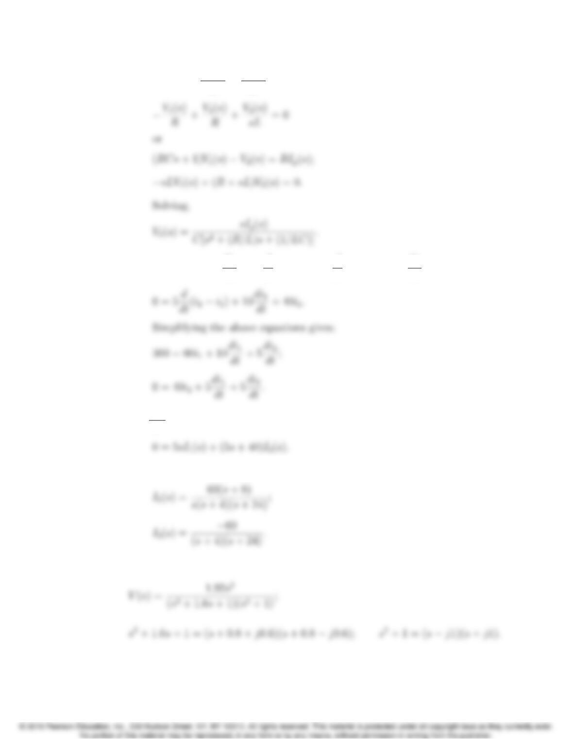
P 12.32 [a] 300 = 60i1+25di1
dt +10d
dt(i2−i1)+5d
dt(i1−i2)−10di1
dt ;
[b] 300
s= (105s+ 60)I1(s)+5sI2(s);
[c] Solving the equations in (b),
P 12.33 From Problem 12.26:
12–20 CHAPTER 12. Introduction to the Laplace Transform
Therefore
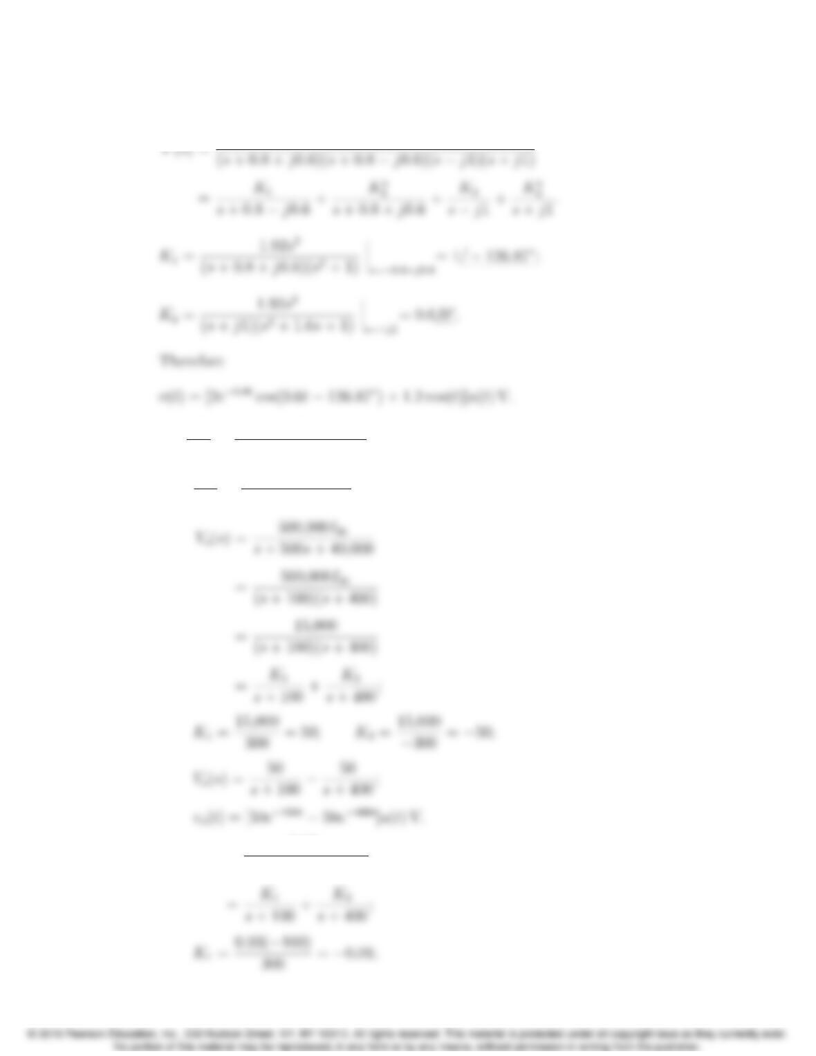
P 12.34 [a] 1
RC =1
(1 ×10³)(2 ×10⁶)= 500;
1
LC =1
(12.5)(2 ×10⁶)= 40,000;
[b] Io(s)= 0.03s
(s+ 100)(s+ 400)
Problems 12–21
K2=0.03(−400)
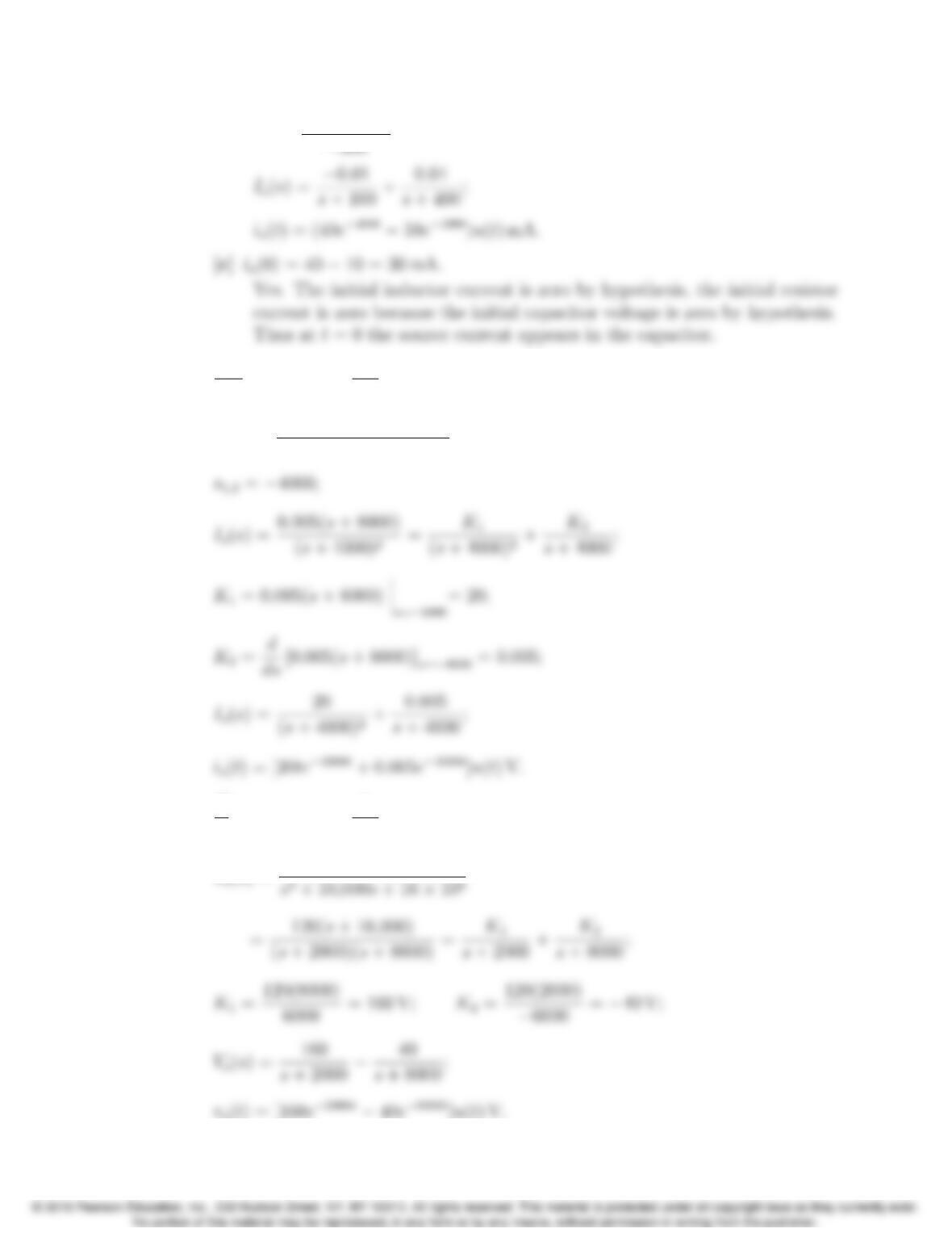
P 12.35 1
RC = 8000; 1
LC = 16 ×106;
Io(s)= 0.005(s+ 8000)
s2+ 8000s+16×106;
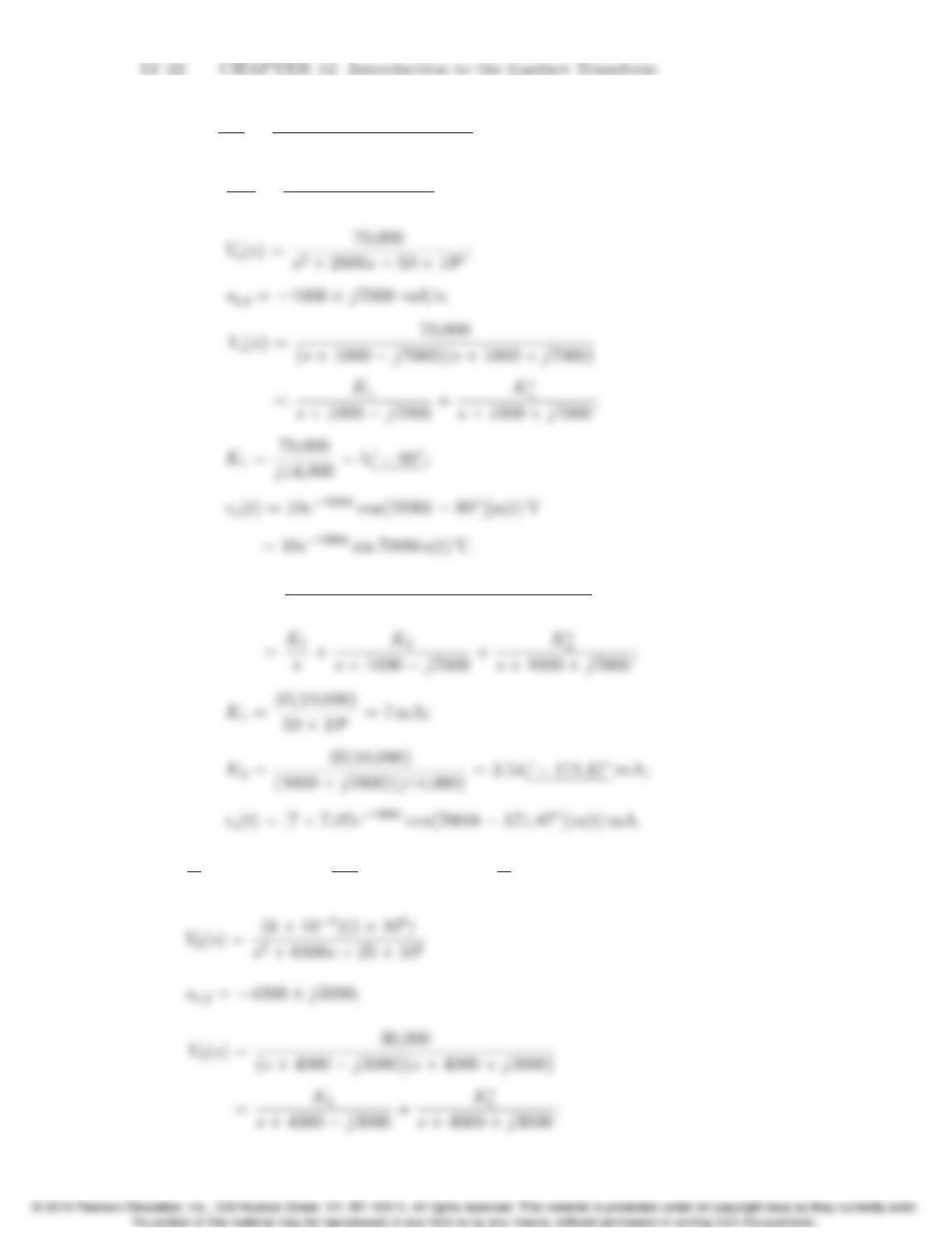
P 12.36 R
L= 10,000; 1
LC = 16 ×106;
Vo(s)= 120(s+10,000)
P 12.37 [a] 1
LC =1
(200 ×103)(100 ×109)= 50 ×106;
1
RC =1
(5000)(100 ×109)= 2000;
[b] Io(s)= 35(10,000)
s(s+ 1000 −j7000)(s+ 1000 + j7000)
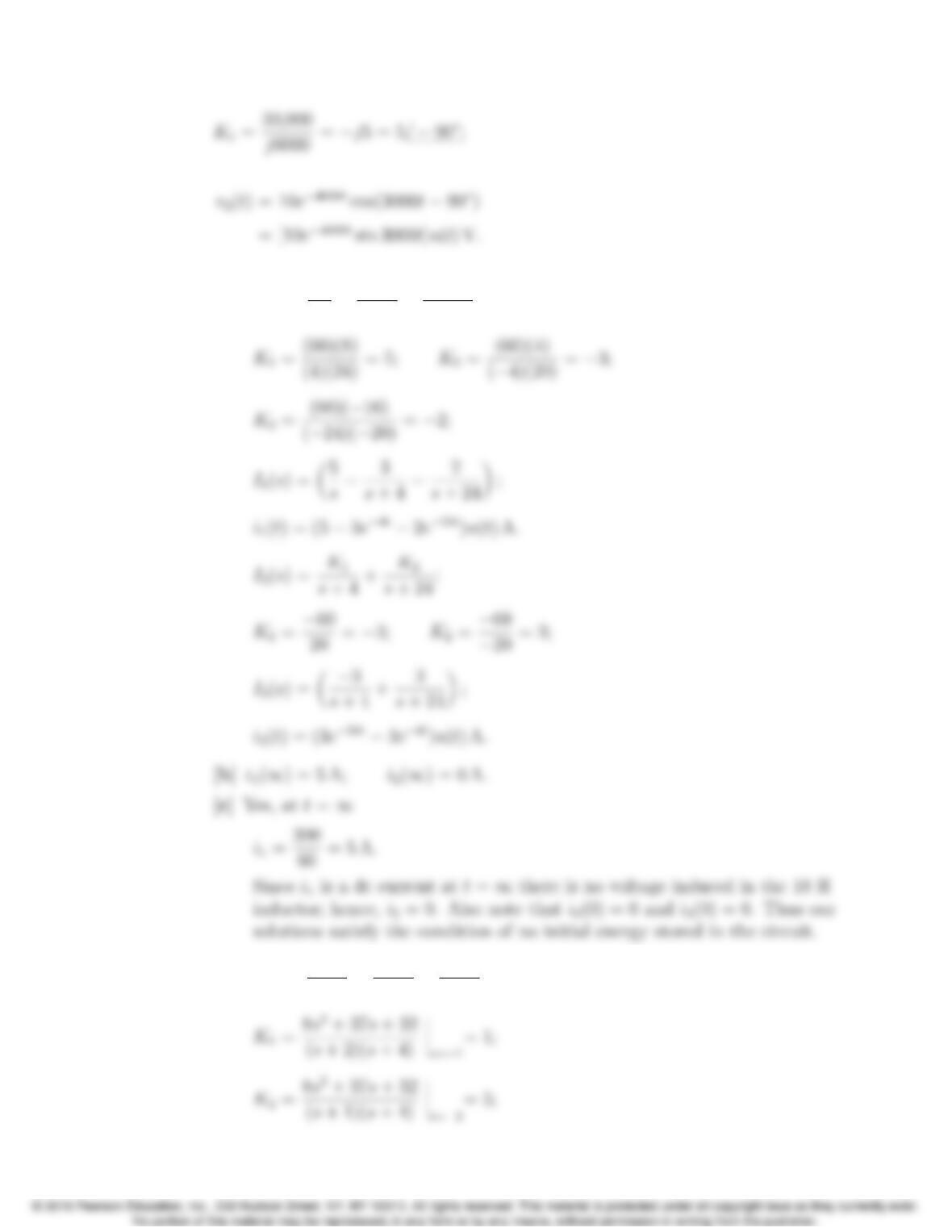
P 12.38 1
C=5×10⁶;1
LC = 25 ×106;R
L= 8000;
Problems 12–23
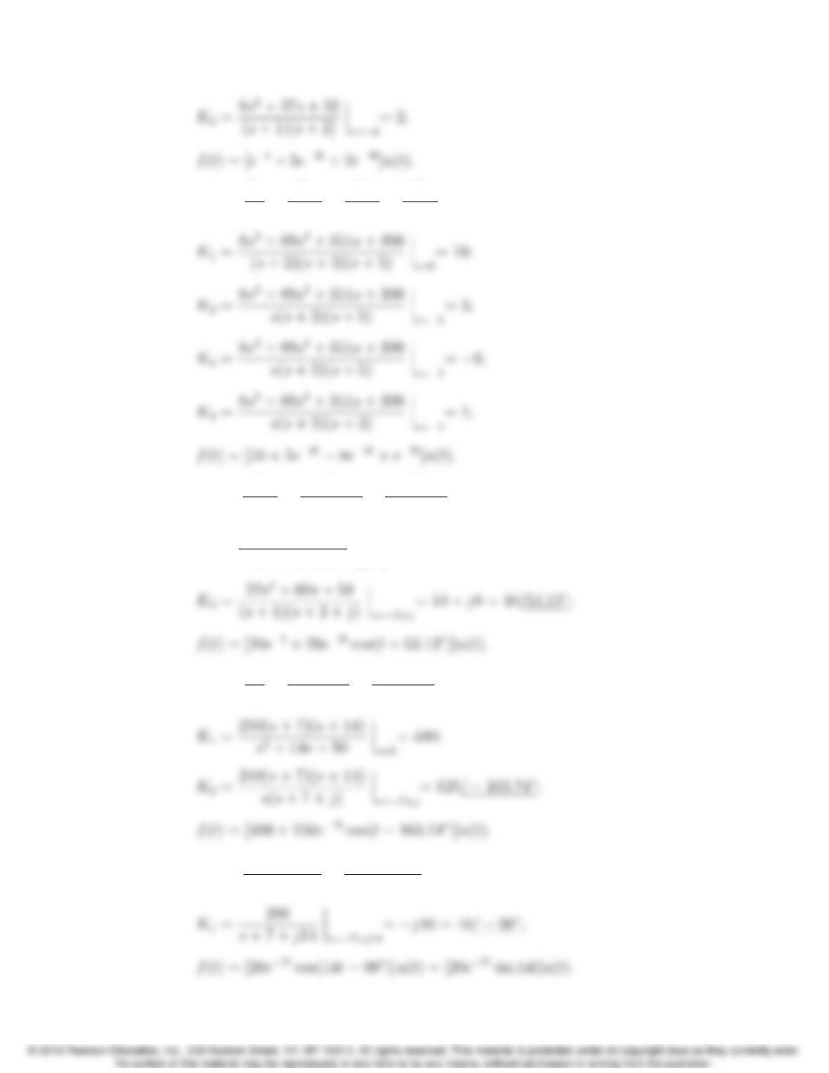
P 12.39 [a] I1(s)=K1
s+K2
s+4+K3
s+24;
P 12.40 [a] F(s)= K1
s+1+K2
s+2+K3
s+4;
12–24 CHAPTER 12. Introduction to the Laplace Transform
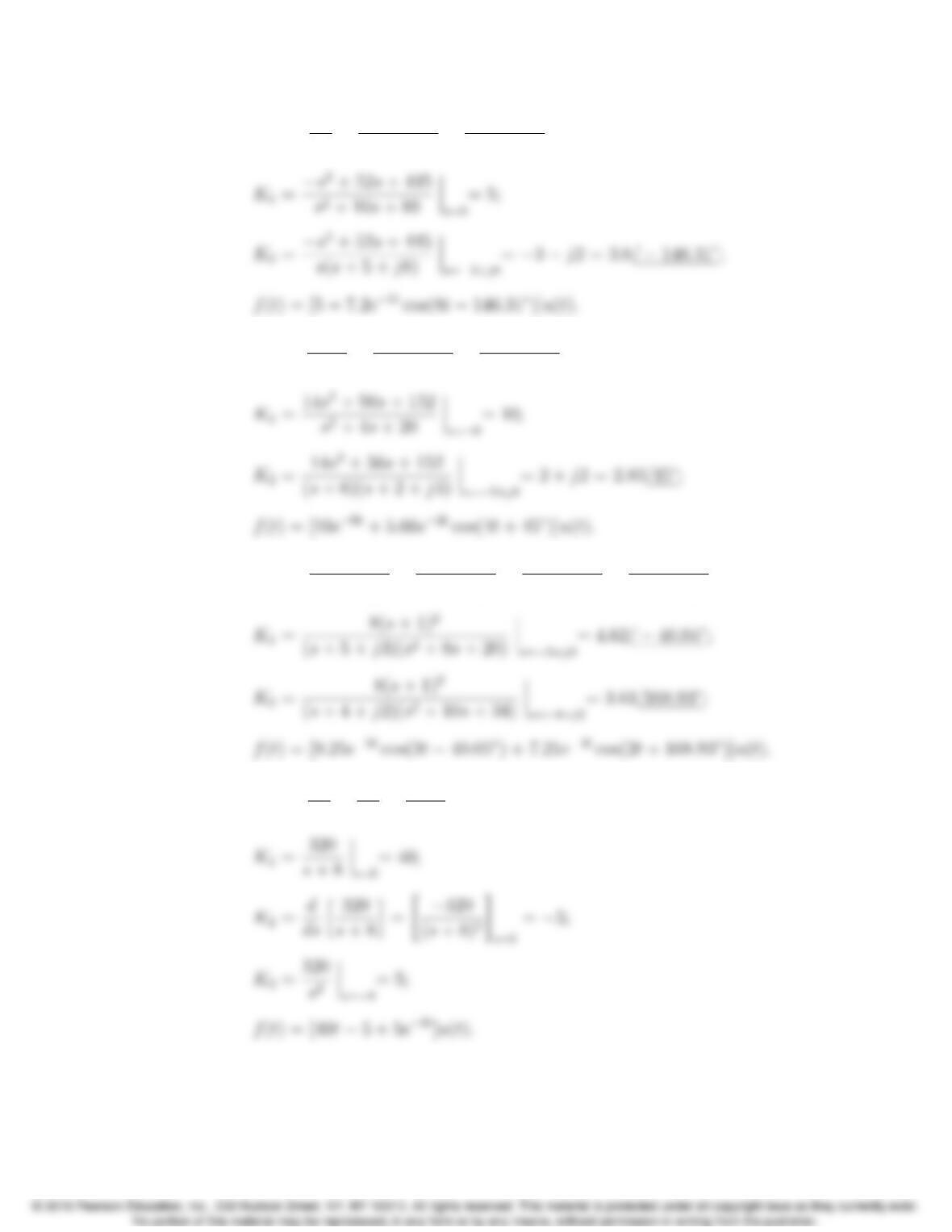
[b] F(s)=K1
s+K2
s+2+K3
s+3+K4
s+5;
[c] F(s)= K1
s+1+K2
s+2−j+K⇤
2
s+2+j;
K1=22s2+60s+58
s2+4s+5 s=1
= 10;
[d] F(s)=K1
s+K2
s+7−j+K⇤
2
s+7+j;
P 12.41 [a] F(s)= K1
s+7−j14 +K⇤
1
s+7+j14;
Problems 12–25
[b] F(s)=K1
s+K2
s+5−j8+K⇤
2
s+5+j8;
[c] F(s)= K1
s+6+K2
s+2−j4+K⇤
2
s+2+j4;
[d] F(s)= K1
s+5−j3+K⇤
1
s+5+j3+K2
s+4−j2+K⇤
2
s+4+j2;
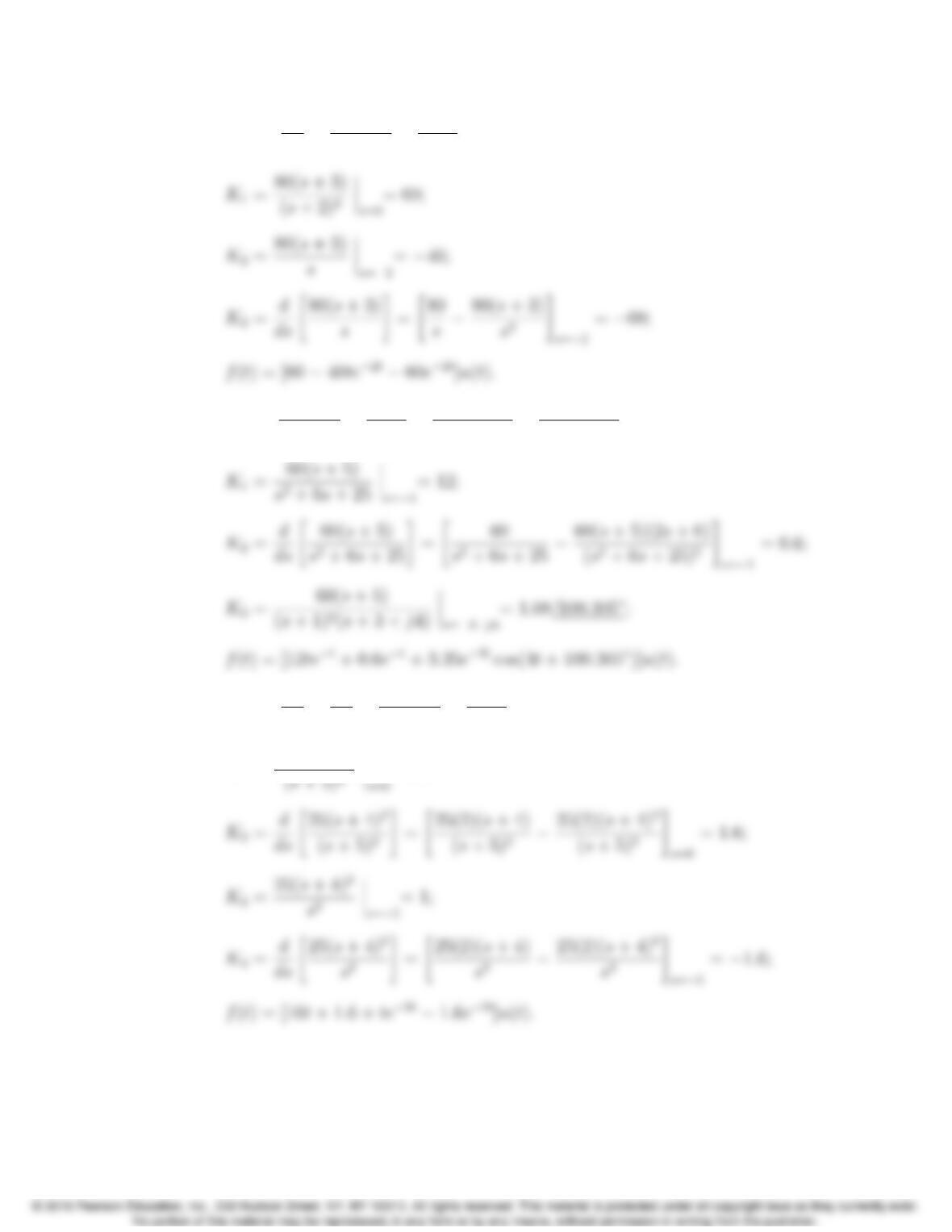
P 12.42 [a] F(s)=K1
s2+K2
s+K3
s+8;
12–26 CHAPTER 12. Introduction to the Laplace Transform
[b] F(s)=K1
s+K2
(s+2)
2+K3
s+2;
[c] F(s)= K1
(s+1)
2+K2
s+1+K3
s+3−j4+K⇤
3
s+3+j4;
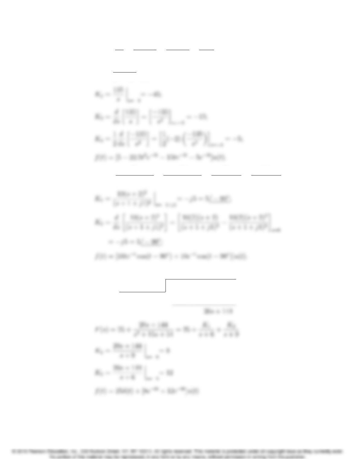
[d] F(s)=K1
s2+K2
s+K3
(s+5)
2+K4
s+5;
K1=25(s+4)
2
2s=0
= 16;
Problems 12–27
P 12.43 [a] F(s)=K1
s+K2
(s+3)
3+K3
(s+3)
2+K4
s+3;
K1=135
(s+3)
3s=0
= 5;
[b] F(s)= K1
(s+1−j1)2+K⇤
1
(s+1+j1)2+K2
s+1−j1+K⇤
2
s+1+j1;
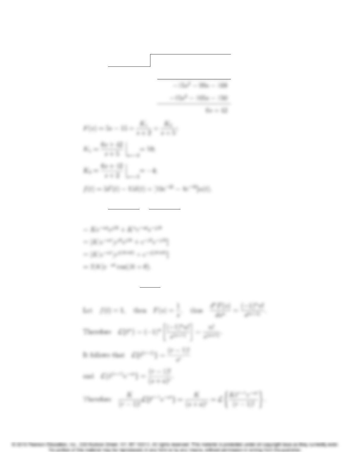
[c] 25
F(s)= s2+15s+54 25s2+ 395s+ 1494
25s2+ 375s+ 1350
12–28 CHAPTER 12. Introduction to the Laplace Transform
[d] 5s−15
F(s)= s2+7s+10 5s3+20s2−49s−108
5s3+35s2+50s
P 12.44 f(t)=L1(K
s+α−jβ+K⇤
s+α+jβ)
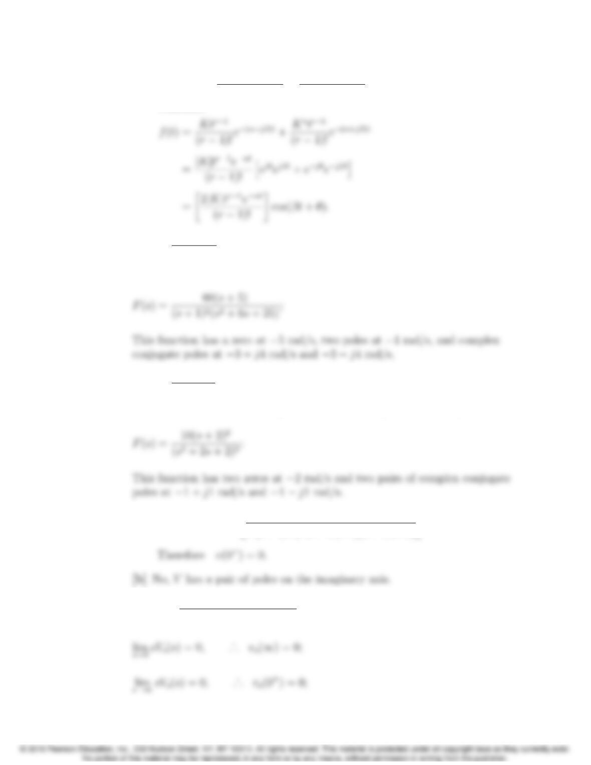
P 12.45 [a] L{tnf(t)}=(−1)n“dnF(s)
dsn#.
Problems 12–29
[b] f(t)=L1(K
(s+α−jβ)r+K⇤
(s+α+jβ)r).
Therefore
P 12.46 F(s)=80(s+3)
s(s+2)
2;
This function has a zero at −3 rad/s, a pole at 0, and two poles at −2 rad/s.
P 12.47 F(s)= 135
s(s+3)
3;
This function has no zeros, a pole at 0, and three poles at −3 rad/s.
P 12.48 [a] lim
s!1 sV (s) = lim
s!1 “1.92s3
s4[1 + (1.6/s) + (1/s2)][1 + (1/s2)]#=0.
P 12.49 sVo(s)= (Idc/C)s
s2+ (1/RC)s+ (1/LC)
12–30 CHAPTER 12. Introduction to the Laplace Transform
sIo(s)= s2Idc
s2+ (1/RC)s+ (1/LC);
P 12.50 sIo(s)= Idcs[s+ (1/RC)]
s2+ (1/RC)s+ (1/LC);
P 12.51 sVo(s)= sVdc/RC
s2+ (1/RC)s+ (1/LC);
lim
s!0sVo(s)=0,·
.. v
o(∞)=0;
P 12.52 [a] sF (s)= 8s3+37s2+32s
(s+ 1)(s+ 2)(s+4);
Problems 12–31
[c] sF (s)= 22s3+60s2+58s
(s+ 1)(s2+4s+5);
P 12.53 [a] sF (s)= 280s
s2+14s+ 245;
s!1 sF (s)=0,·
[b] sF (s)=−s2+52s+ 445
s2+10s+89 ;
[c] sF (s)= 14s3+56s2+ 152s
(s+ 6)(s2+4s+ 20);
P 12.54 [a] sF (s)= 320
s(s+8).
12–32 CHAPTER 12. Introduction to the Laplace Transform
[b] sF (s)=80(s+3)
(s+2)
2;
[c] sF (s)= 60s(s+5)
(s+1)
2(s2+6s+ 25);
[d] sF (s)=25(s+4)
2
s(s+5)
2.
P 12.55 [a] sF (s)= 135
(s+3)
3;
lim
s!0sF (s)=5,·
.. f(∞)=5;
[c] This F(s) function is an improper rational function, and thus the
[d] This F(s) function is an improper rational function, and thus the
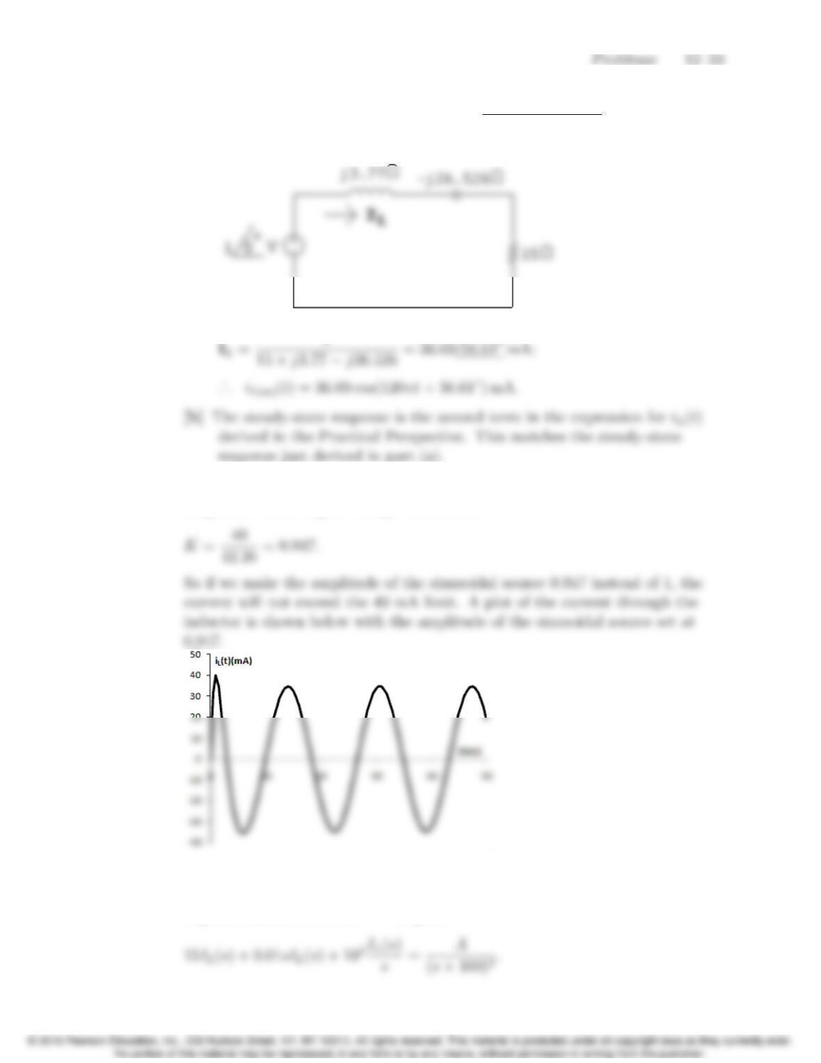
P 12.56 [a] ZL=j120π(0.01) = j3.77 Ω;ZC=−j
120π(100 ×106)=−j26.526 Ω.
The phasor-transformed circuit is
P 12.57 The transient and steady-state components are both proportional to the
magnitude of the input voltage. Therefore,
P 12.58 We begin by using the Laplace transform of the describing differential
equation for the circuit in Fig. 12.19. Change the right-hand side so it is the
Laplace transform of Kte100tto give:
12–34 CHAPTER 12. Introduction to the Laplace Transform
Solving for IL(s),
1
Therefore,
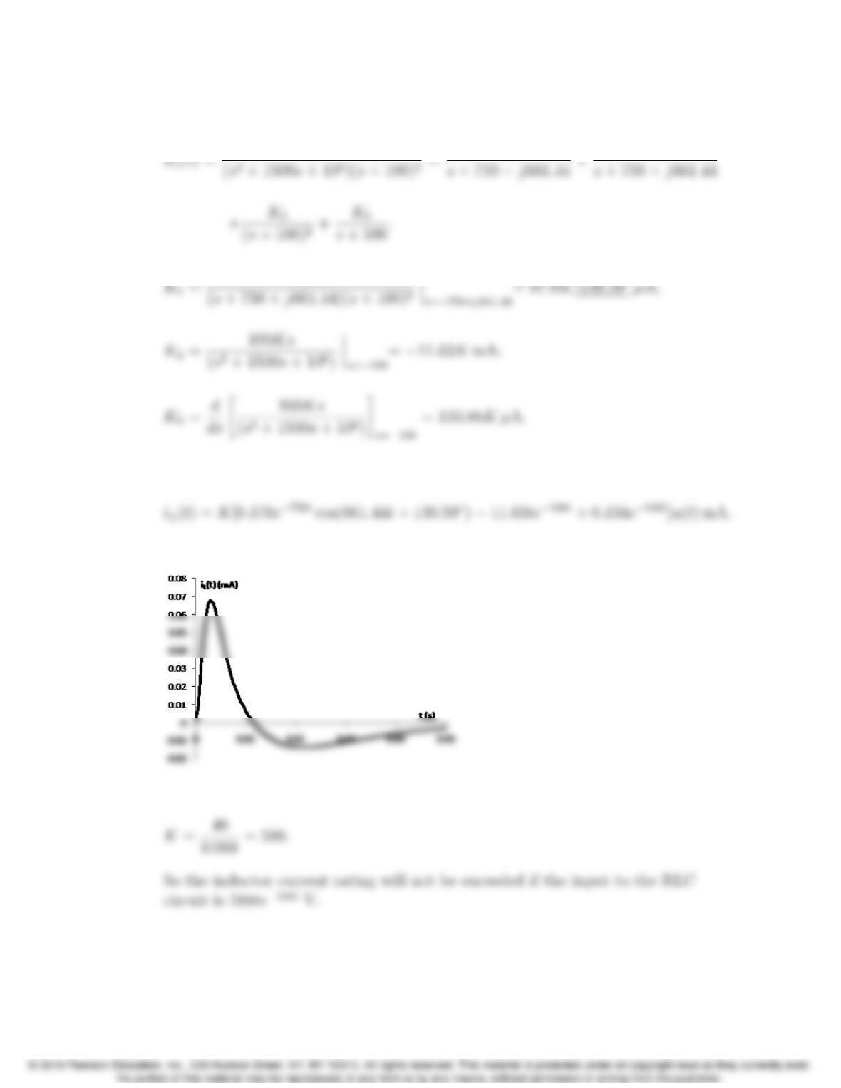
Plot the expression above with K= 1:
The maximum value of the inductor current is 0.068KmA. Therefore,