CHAPTER 10
Exercises
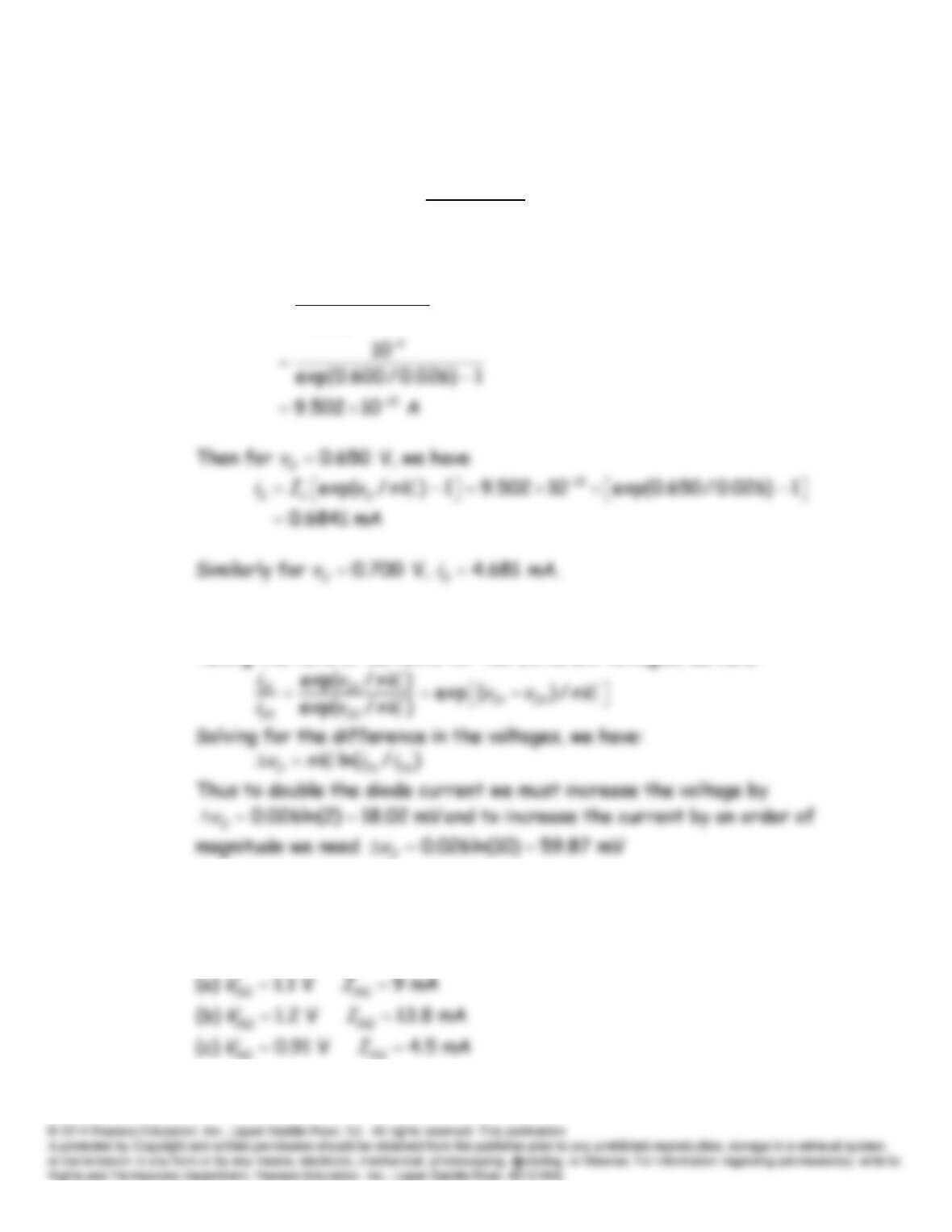
E10.1 Solving Equation 10.1 for the saturation current and substituting values,
we have
exp( / ) 1
D
s
T
D
i
Iv nV
E10.2 The approximate form of the Shockley Equation is
exp( / )
sT
DD
i I v nV
.
Taking the ratio of currents for two different voltages, we have
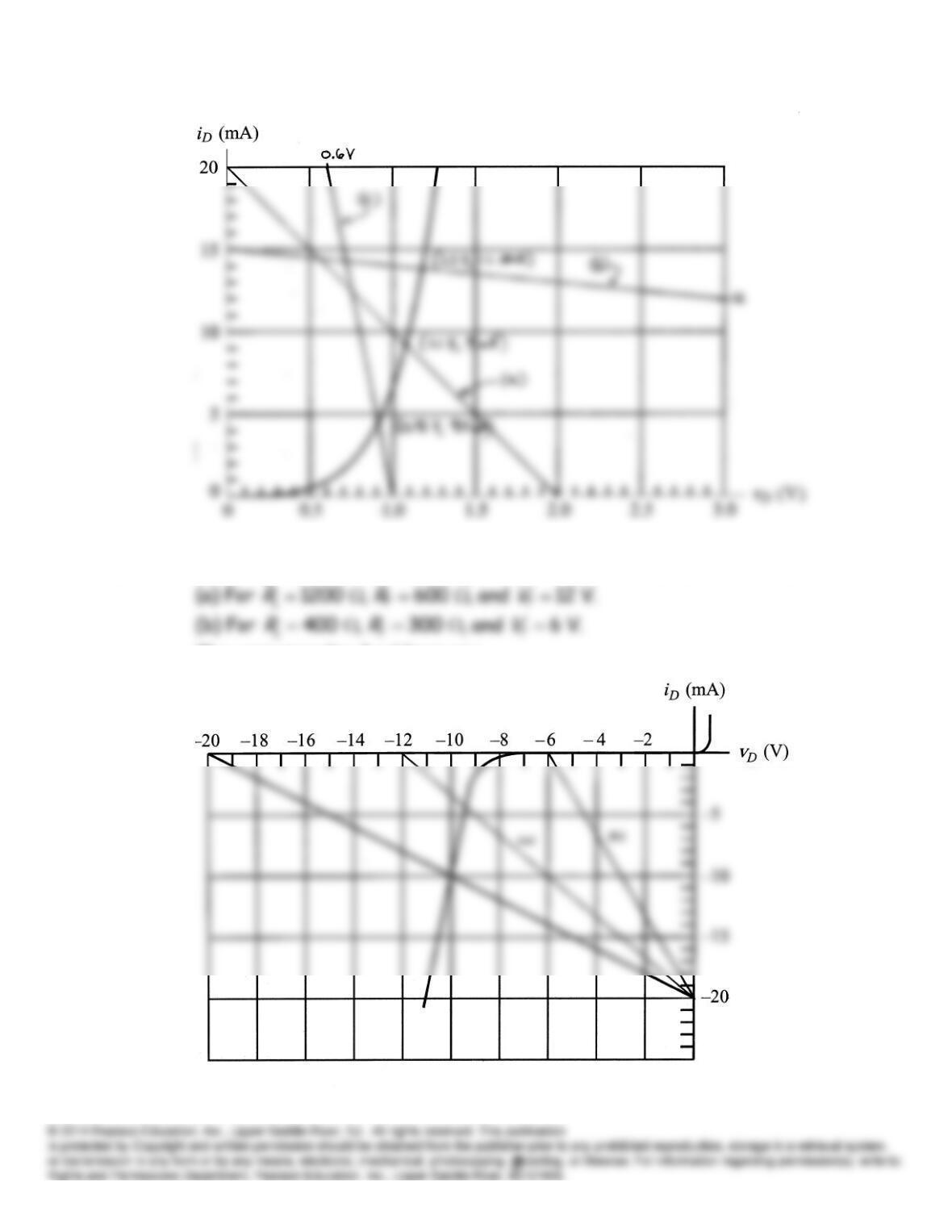
E10.3 The load line equation is
.
SS DD
V Ri v
The load-line plots are shown on
the next page. From the plots we find the following operating points:
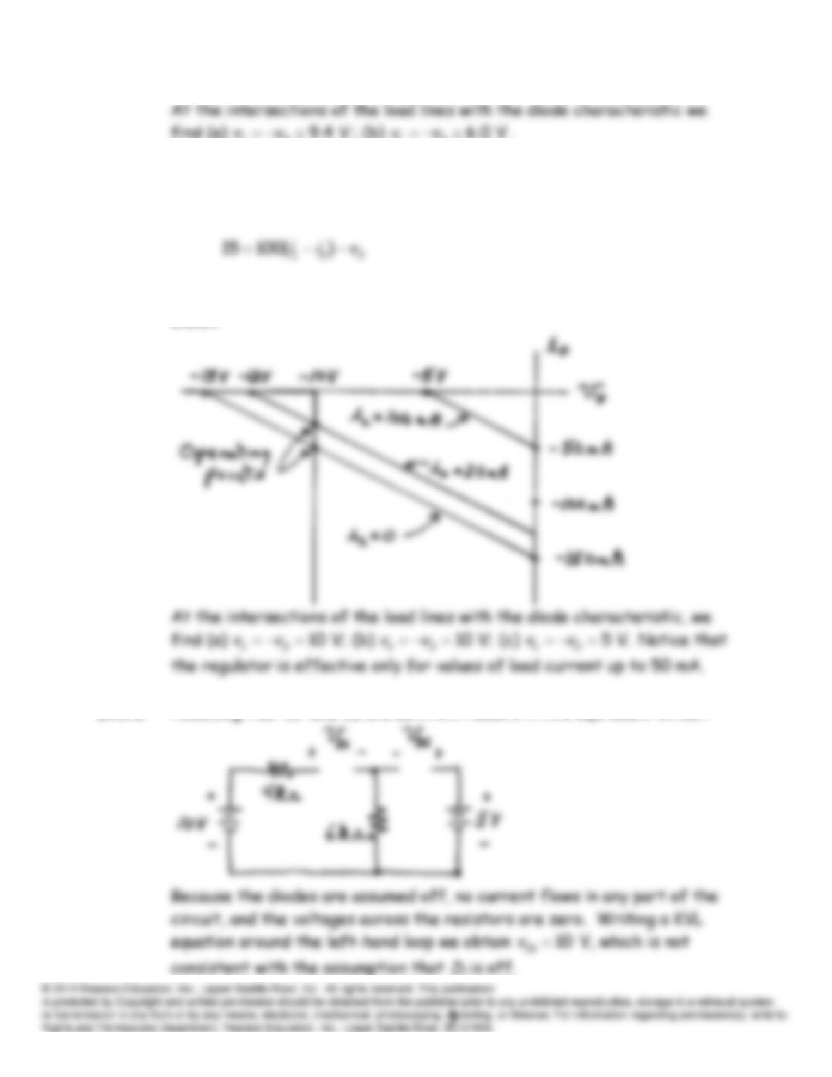
E10.4 Following the methods of Example 10.4 in the book, we determine that:
The corresponding load lines are:
LD
LD
E10.5 Writing a KVL equation for the loop consisting of the source, the
resistor, and the load, we obtain:
The corresponding load lines for the three specified values of
iL
are
shown:
E10.6 Assuming that
D
and
D
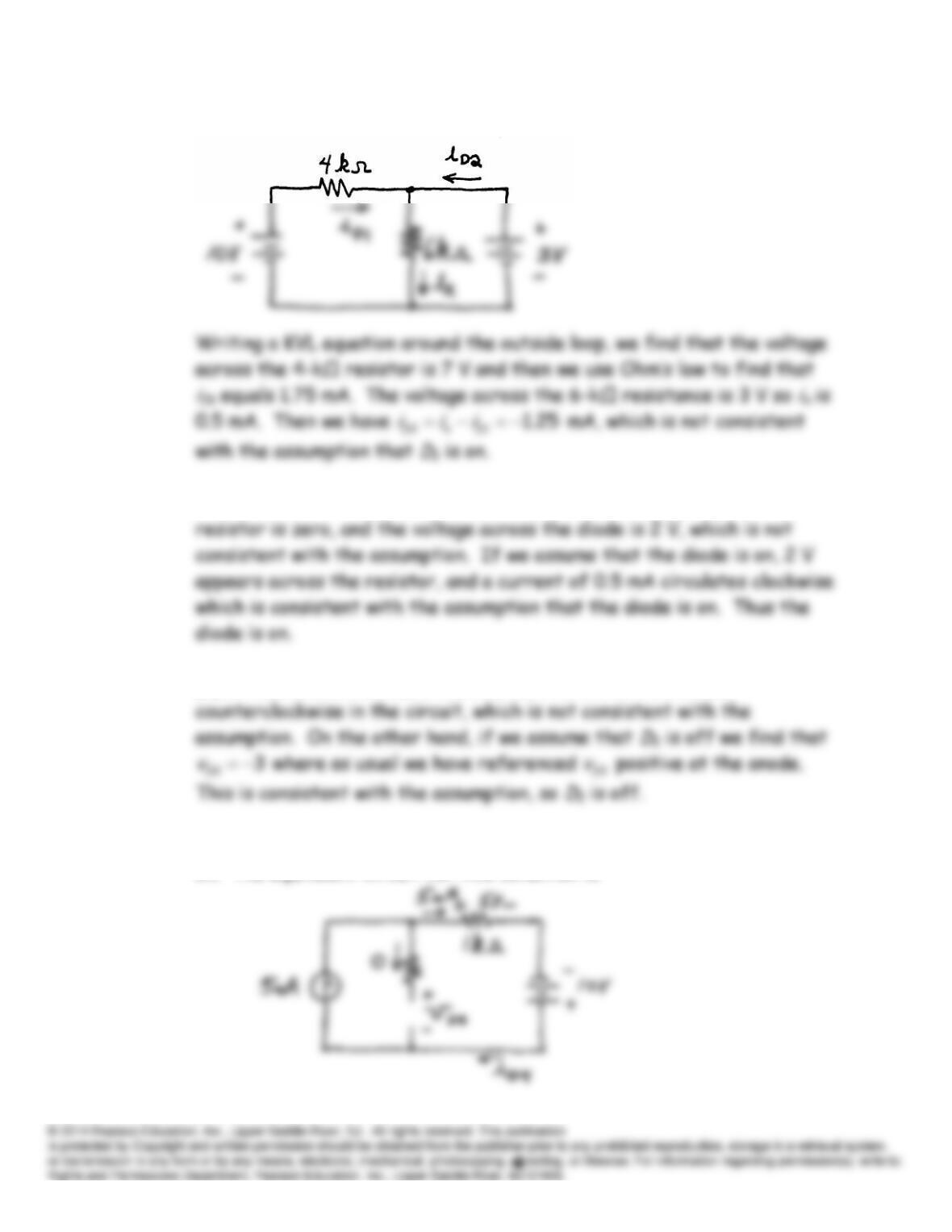
E10.7 Assuming that
D
1
and
D
2 are both on results in this equivalent circuit:
E10.8 (a) If we assume that
D
1 is off, no current flows, the voltage across the
(b) If we assume that
D
2 is on, a current of 1.5 mA circulates
(c) It turns out that the correct assumption is that
D
3 is off and
D
4 is
on. The equivalent circuit for this condition is:
E10.9 (a) With
RL
= 10 kΩ, it turns out that the diode is operating on line
segment
C
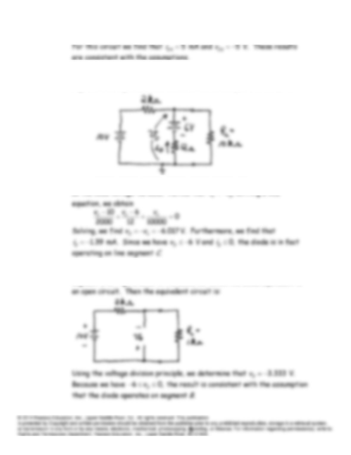
of Figure 10.19 in the book. Then the equivalent circuit is:
We can solve this circuit by using the node-voltage technique, treating
vo
as the node voltage-variable. Notice that
.
vv
Writing a KCL
(b) With
RL
= 1 kΩ, it turns out that the diode is operating on line
segment
B
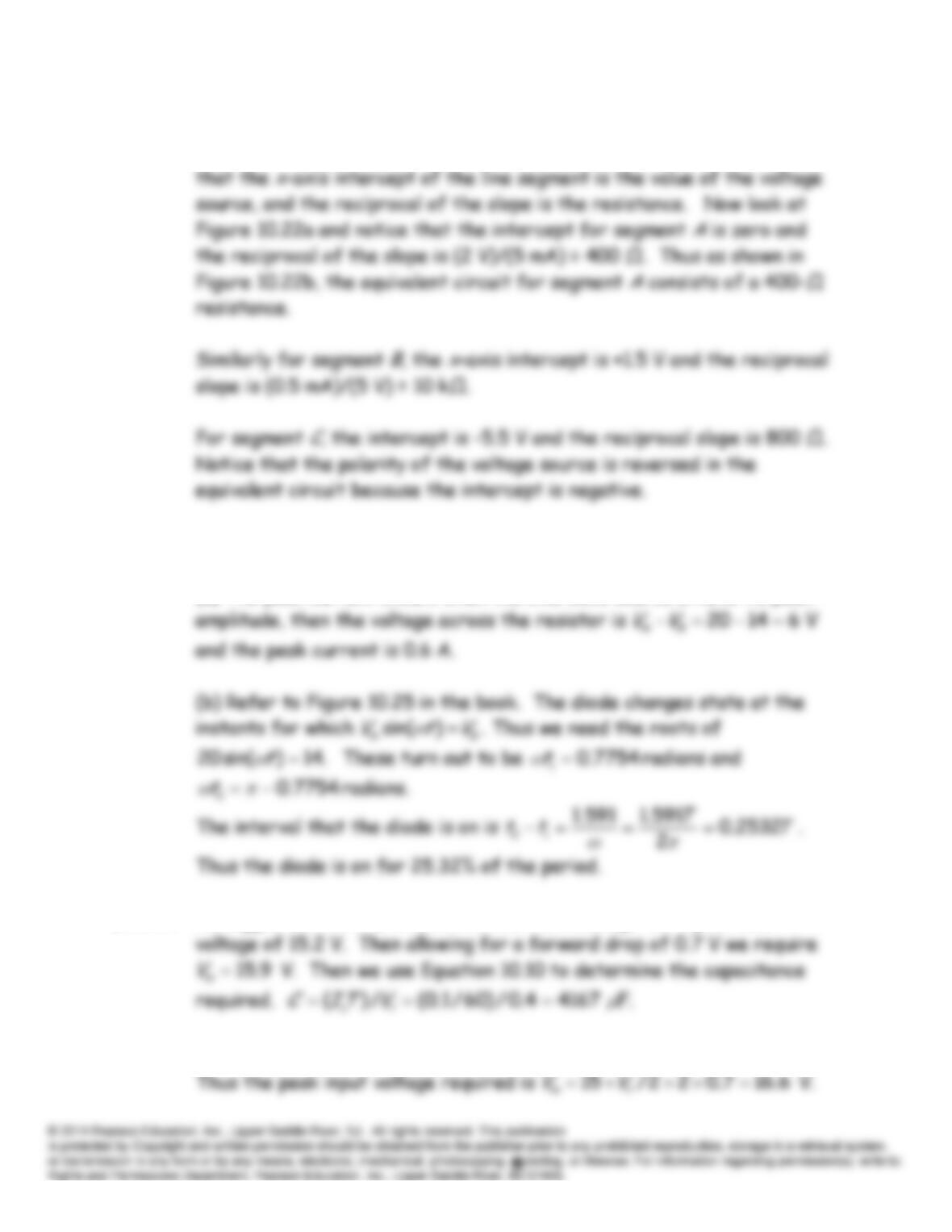
of Figure 10.19 in the book, for which the diode equivalent is
E10.10 The piecewise linear model consists of a voltage source and resistance in
series for each segment. Refer to Figure 10.18 in the book and notice
E10.11 Refer to Figure 10.25 in the book.
(a) The peak current occurs when the sine wave source attains its peak
E10.12 As suggested in the Exercise statement, we design for a peak load
E10.13 For the circuit of Figure 10.28, we need to allow for two diode drops.
E10.14 Refer to Figure 10.31 in the book.
(a) For this circuit all of the diodes are off if
1.8 10
o
v
. With the
in.
o
(b) ) For this circuit both diodes are off if
55
o
v
. With the diodes
off, no current flows and
in.
o
vv
in
o
E10.16 Refer to Figure 10.34a in the book.
(a) If
in( ) 0,
vt
we have only a dc source in the circuit. In steady state,
in.
E10.18 One design is shown in Figure 10.36. Other correct answers are possible.
E10.19 Equation 10.22 gives the dynamic resistance of a semiconductor diode as
/
TDQ
d
r nV I
.
0.1
26,000
10
26
E10.20 For the
Q
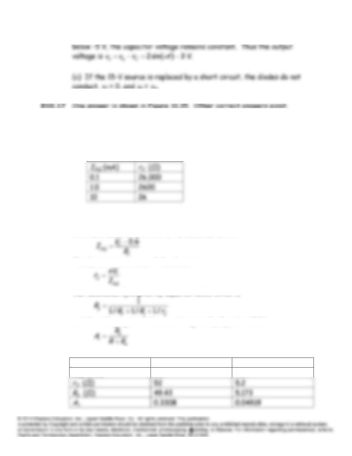
-point analysis, refer to Figure 10.42 in the book. Allowing for
a forward diode drop of 0.6 V, the diode current is
The dynamic resistance of the diode is
the resistance
Rp
is given by Equation 10.23 which is
and the voltage gain of the circuit is given by Equation 10.24.
Evaluating we have
VC
(V)
1.6
10.6
IDQ
(mA)
0.5
5.0
52
5.2
(Ω)
49.43
5.173
Problems
P10.3
P10.4 The Shockley equation gives the diode current
D
i
in terms of the applied
voltage
D
v
:
P10.5
)1060.1/()1038.1(/ 1923
TqkTVT
P10.6 For
D
v
0.6 V, we have
Thus, we determine that:
P10.7* The approximate form of the Shockley Equation is
exp( / )
sT
DD
i I v nV
.
Taking the ratio of currents for two different voltages, we have
Solving for
n
we obtain:
P10.9
P10.11
mV 17.32)1060.1/()3731038.1(/ 1923
qkTVT
P10.12 Using the approximate form of the Shockley Equation, we have
3
10 exp 0.600
sT
I nV
(1)
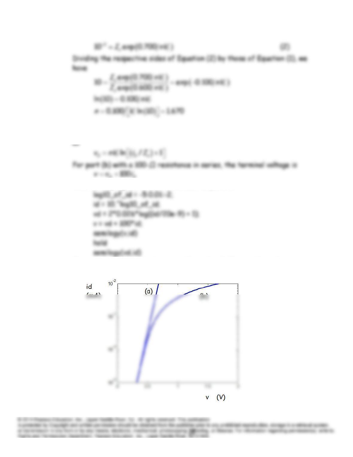
P10.13 For part (a), Equation 10.3 gives the diode voltage in terms of the current
DD ivv
A MATLAB program to obtain the desired plots is:
(Note in MATLAB log is the natural logarithm.) The resulting plots are
shown:
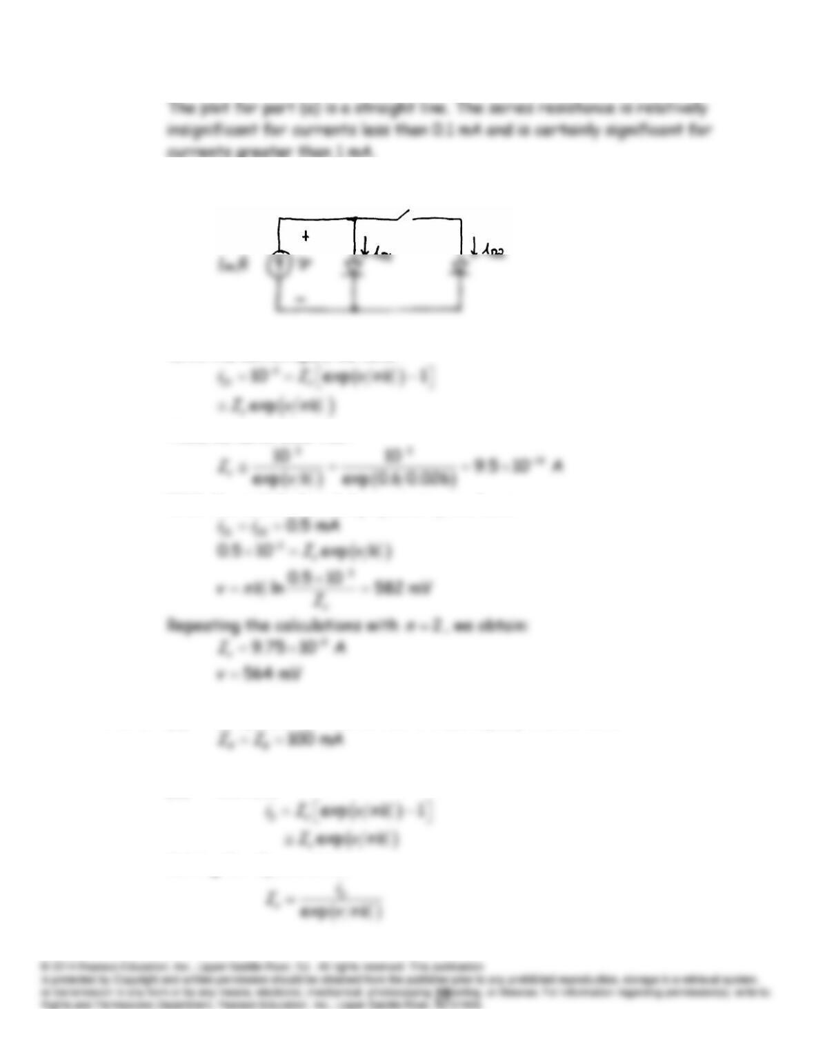
P10.14*
With the switch open, we have:
Thus, we determine that:
With the switch closed, by symmetry, we have:
P10.15* (a) By symmetry, the current divides equally and we have
(b) We have
Solving for
s
I
, we obtain
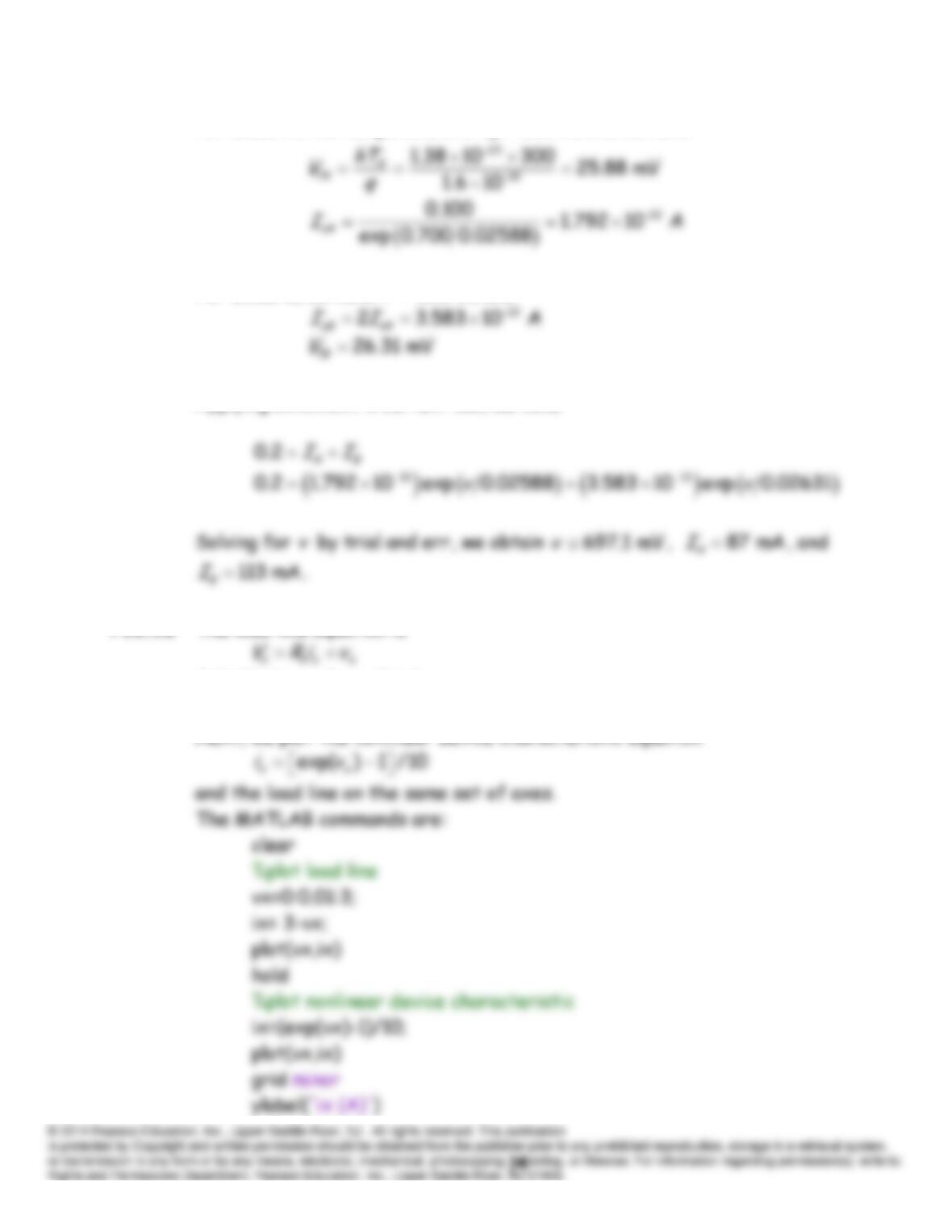
For diode
A
, the temperature is
300 K
T
, and we have
For diode
B
, we have
305 K
T
, and
Applying Kirchhoff’s current law, we have
P10.16* The load-line equation is
Substituting values, this becomes
3
xx
iv
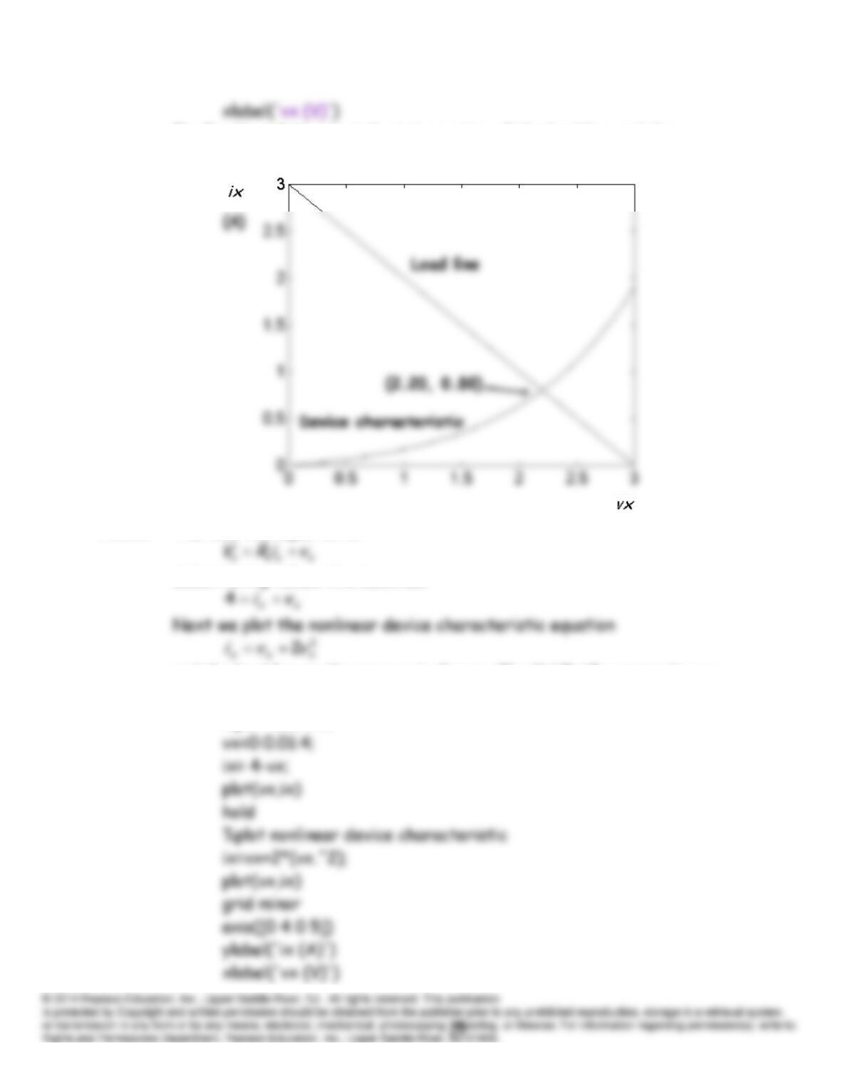
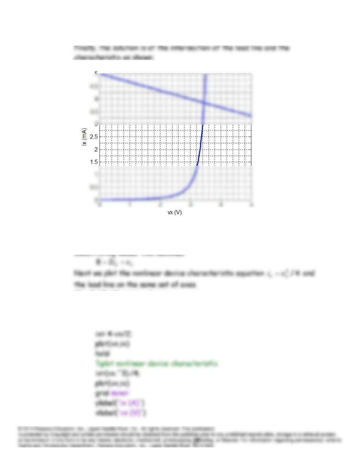
Finally, the solution is at the intersection of the load line and the
characteristic as shown:
P10.17 The load-line equation is
Substituting values this becomes
and the load line on the same set of axes. The MATLAB commands are:
clear
%plot load line
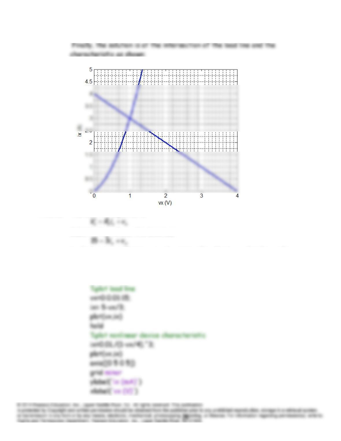
P10.18 The load-line equation is
Substituting values, this becomes
in which
ix
is in milliamperes and
vx
is in volts. Next, we plot the nonlinear
device characteristic equation and the load line on the same set of axes
using the commands:
clear
P10.19 The load line equation is
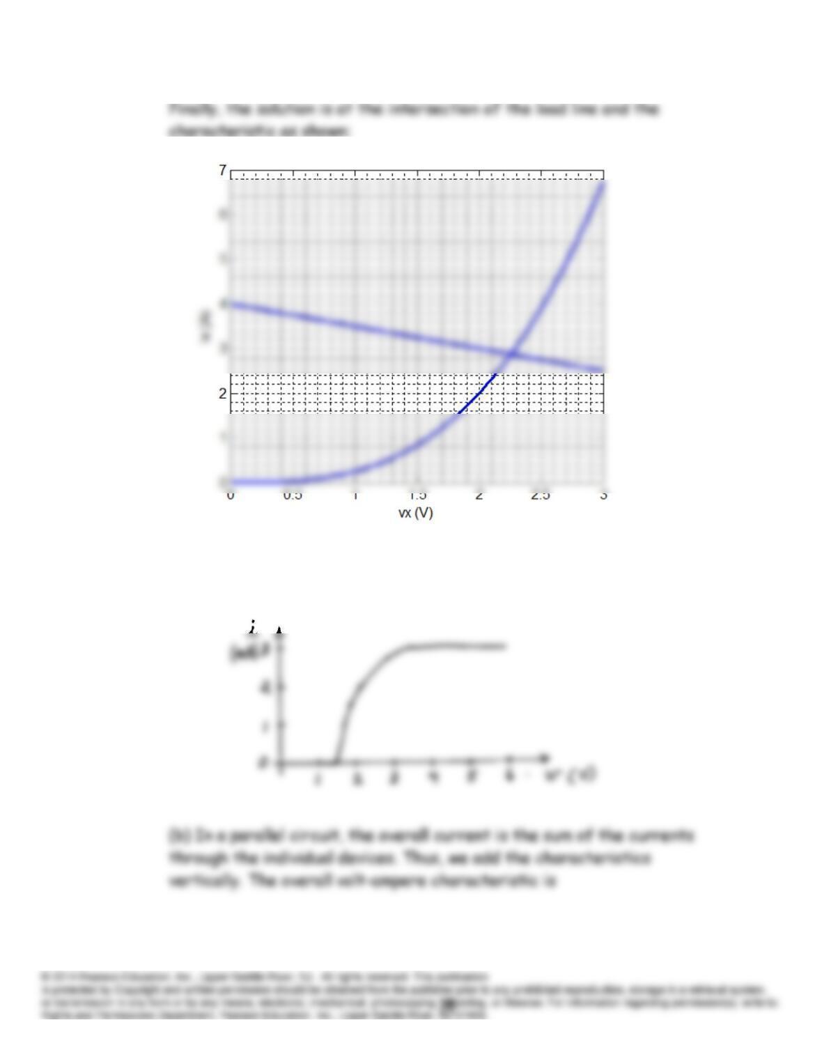
s s x x
V R i v
The MATLAB commands are:
clear
%plot load line
vx=0:0.01:3;
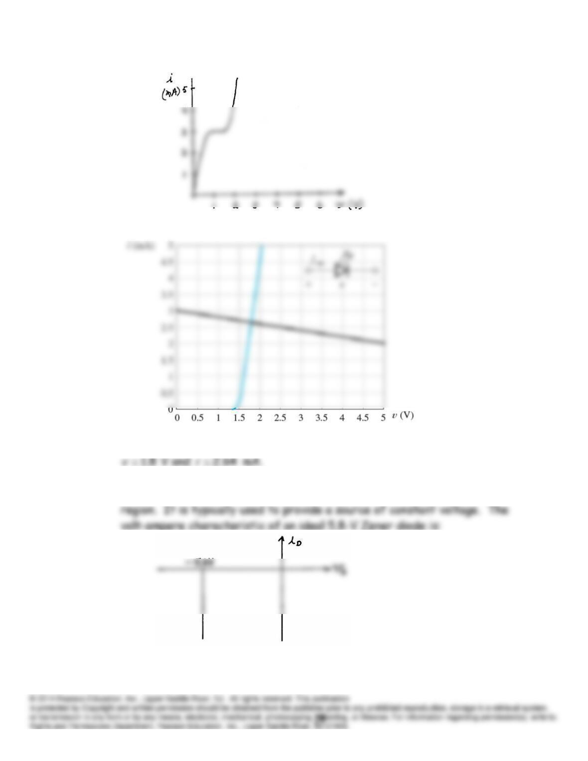
P10.20 (a) In a series circuit, the total voltage is the sum of the voltages across
the individual devices. Thus, we add the characteristics horizontally. The
overall volt-ampere characteristic is
P10.21 The load-line construction is:
At the intersection of the characteristic and the load line, we have
P10.22 A Zener diode is a diode intended for operation in the reverse breakdown
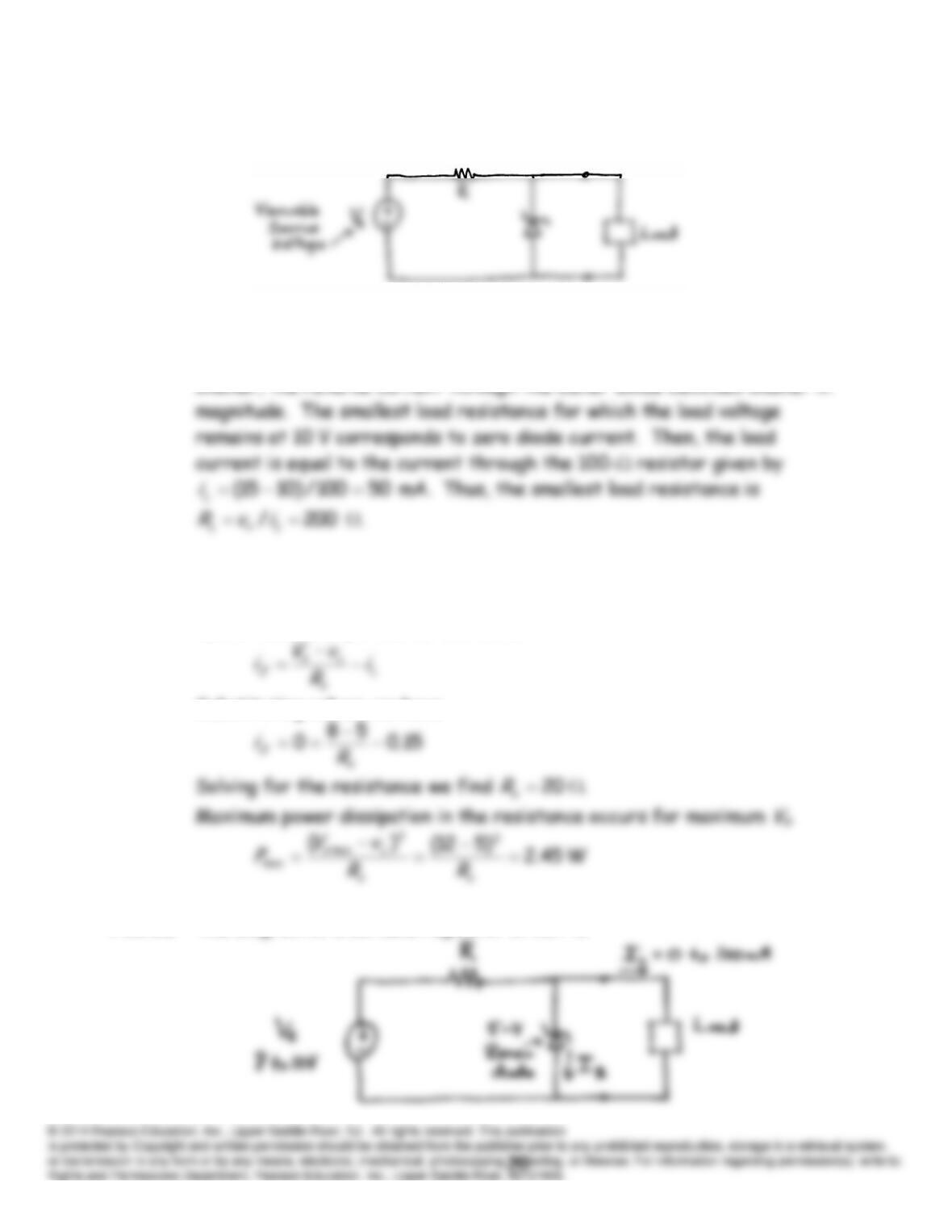
P10.23* The circuit diagram of a simple voltage regulator is:
P10.24 Refer to Figure 10.14 in the book. As the load resistance becomes
P10.25 We need to choose
Rs
so the minimum reverse current through the Zener
diode is zero. Minimum current through the Zener occurs with minimum
Vs
and maximum
iL
. Also, we can write:
Substituting values, we have
P10.26 The diagram of a suitable regulator circuit is