Page 5 of 5 MATLAB Project: Using Eigenvalues to Study Spotted Owls
(c) Prove that the real eigenvalue 1
λ
is greater than 23
||||
λλ
=. Hence, the real positive
eigenvalue of A will always be the dominant eigenvalue for this type matrix.
MATLAB Project: QR Factorization Name_______________________________
Purpose: To learn to use MATLAB’s qr function and understand the connections between the
matrices it produces and the QR factorization described in the text
Prerequisite: Section 6.4
MATLAB functions used: qr; and gs and qrdat from Laydata4 Toolbox
Background. In MATLAB, the command [Q R]=qr(A) works for any shape matrix A. It creates a
square matrix Q whose columns are orthonormal (up to machine accuracy) and a matrix R which is the
same shape as A and “upper triangular.” Furthermore, A = QR (up to machine accuracy), and this is called
a QR factorization of A.
1. Verify the statements above for each matrix below. To get you started, type qrdat to get the matrices,
then type [Q R]=qr(A) and record Q and R beside A below. Notice Q is square and R has the same
shape as A and is “upper triangular.”
Check that the columns of Q are orthonormal by using Theorem 6 in section 6.2. Type format
long, Q’*Q and inspect to see that this product looks essentially like an identity matrix. Also compare
378
−
⎣⎦
35
−
⎡⎤
⎢⎥
143
147
C
⎢⎥
=−−
⎢⎥
−
⎢⎥
Q= R=
Page 2 of 3 MATLAB Project: QR Factorization
Background. The QR factorization developed in Section 6.4 of Lay’s text is somewhat different from the
factorization produced by MATLAB’s qr function. Recall how Lay’s algorithm works: A must have
independent columns (so A must be square or “tall”). The Gram-Schmidt Process is applied to the
columns of A; this yields a matrix 1
Q the same shape as A whose columns are orthonormal, and a square
upper triangular matrix 11
QR such that 11
A
QR=is true. So if A is not square, 1
Qand 1
R
are clearly different
from the Q and R you get from executing [Q R]=qr(A)since they have different shapes.
2. (hand) Using the matrix C above, investigate the connection between the matrices produced by the
text’s QR factorization algorithm and the matrices produced by the qr function. In more detail:
3. (MATLAB) The function gs does the Gram-Schmidt Process as described in Theorem 11, Section 6.4.
To verify this, type G = gs(C) and record G:
G =
(b) How does G compare to the matrix 1
Qthat you calculated by hand in question 2(a)?
4. (hand) Let A be an mn×matrix, let 12
,,,
k
PP P…be mm×orthogonal matrices, let 21k
R
PPPA=and
let 21
()
T
k
QPPP=. Explain why Q must be an orthogonal matrix and why A must equal QR. You may
cite theorems from the text. Attach an extra sheet.
5.2.) The idea is to create a sequence of matrices similar to A which converges to an upper triangular
matrix. If this can be done then the diagonal entries of the limit matrix are the eigenvalues of A. The
remarkable discoveries are that the method can be done with great accuracy, and it will converge for
1. (hand) Here you will verify some of the basic matrix properties that underlie this modern method.
Suppose A is nn×. Let 00
AQR= be a QR factorization of A and create 100
A
RQ=. Let 111
A
QR= be a QR
factorization of 1
A
and create 211
ARQ=. Explain why the following are true; use your paper and attach:
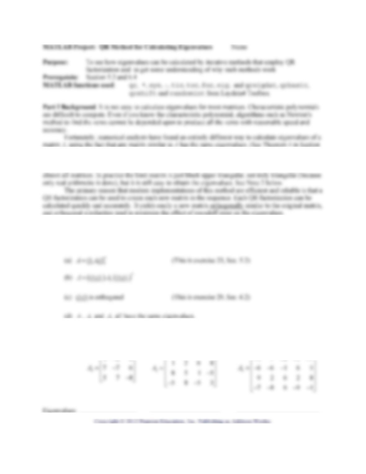
2. (MATLAB) Type qreigdat to get the following matrices. Then use MATLAB’s eig function to
calculate their eigenvalues, and record their eigenvalues below each matrix:
⎢
⎢
⎢
⎢
⎣
⎢
⎢
⎢
⎢
⎢
⎣
128
−
4237
−
⎡
⎤
26349
17 4 37
−−
⎡
⎤
⎢
⎥
−−−−
Page 2 of 6 MATLAB Project: QR Method for Calculating Eigenvalues
00 14 16
022525
−−−
⎡⎤
⎢⎥
−−−−
⎢⎥
Part II: The basic QR algorithm.
Definition. The basic QR algorithm for eigenvalues is the iterative process begun in question 1, repeated
many times: let 00
AQR=be a QR factorization of A and create 100
ARQ=. Let 111
AQR= be a QR
factorization of 1
Aand create 211
ARQ=. Continue the process of having created m
A, let mmm
AQR=be a
3. (MATLAB) For each of the matrices shown above, use the function qrbasic to find how many steps
of the basic QR algorithm are needed to make the absolute value of every entry below the diagonal
smaller than 0.001, and how many seconds this takes. In the first column of the table on page 4, record the
number of steps, the time, and the final matrix.
The function qrbasic simply does the commands [Q R]=qr(A),A=R*Q repeatedly. The
program will stop when all entries below the diagonal are smaller than 0.001 (or after 200 steps if that test
Part III: Improving the basic QR algorithm by shifting and deflating
It is true that the basic algorithm can fail to converge for some matrices, and even when it does
converge it can be extremely slow. There are simple modifications which greatly speed it up and can also
make it converge for more matrices.
One of these modifications is shifting. If A is the original matrix and m
A
is the current matrix in
the iteration, choose a scalar c, then get a QR factorization of the shifted matrix m
AcI−, and then undo
4. (hand) Let A be nn×, let I denote the nn× identity matrix, and let c be a constant.
(a) Let
λ
be an eigenvalue of A. Explain why A
λ
=xx
is true if and only if ()()AcI c
λ
−=−xx
(b) Let AcI QR−= be a QR factorization of
A
cI−, and define 1
ARQcI=+
.
Show that 1
T
A
QA Q=.
(c) Suppose
B
C
AOD
⎡⎤
=⎢⎥
, where B and D are square and O is a zero matrix. Explain why the
Definition. The QR algorithm for eigenvalues using diagonal shifts is the following iterative
process. Repeat the step described in question 4(b), each time choosing the value for the next scalar c to
be the last diagonal entry of the previous matrix k
A
. Stop when the last row of k
A
looks like
[
]
12 k
s
ssx…where each i
s
is very small. Then that last entry x is approximately an eigenvalue of
s
5. (MATLAB) Use the function qrshift to apply the shift-deflate algorithm just described to the four
matrices 3
A,4
A,5
Aand 6
A. You will find how many seconds and how many steps are needed to make the
absolute value of every entry below the diagonal less than 0.001, and then for 0.0001.
The function qrshift does shifting as described in question 4(b), and it deflates after the
entries below the diagonal are less than the tolerance you specify. It will display each deflation, the final
matrix and how many iterative steps were done. To perform the calculations for 3
A, type
Next type tic, qrshift(A3,0.0001),toc , and repeat these calculations for the other
matrices while recording results on page 4.
6. (hand) Based on what you have seen, how does the basic QR method compare with the shift-deflate
QR method? Discuss, use your paper, and attach.
Page 4 of 6 MATLAB Project: QR Method for Calculating Eigenvalues
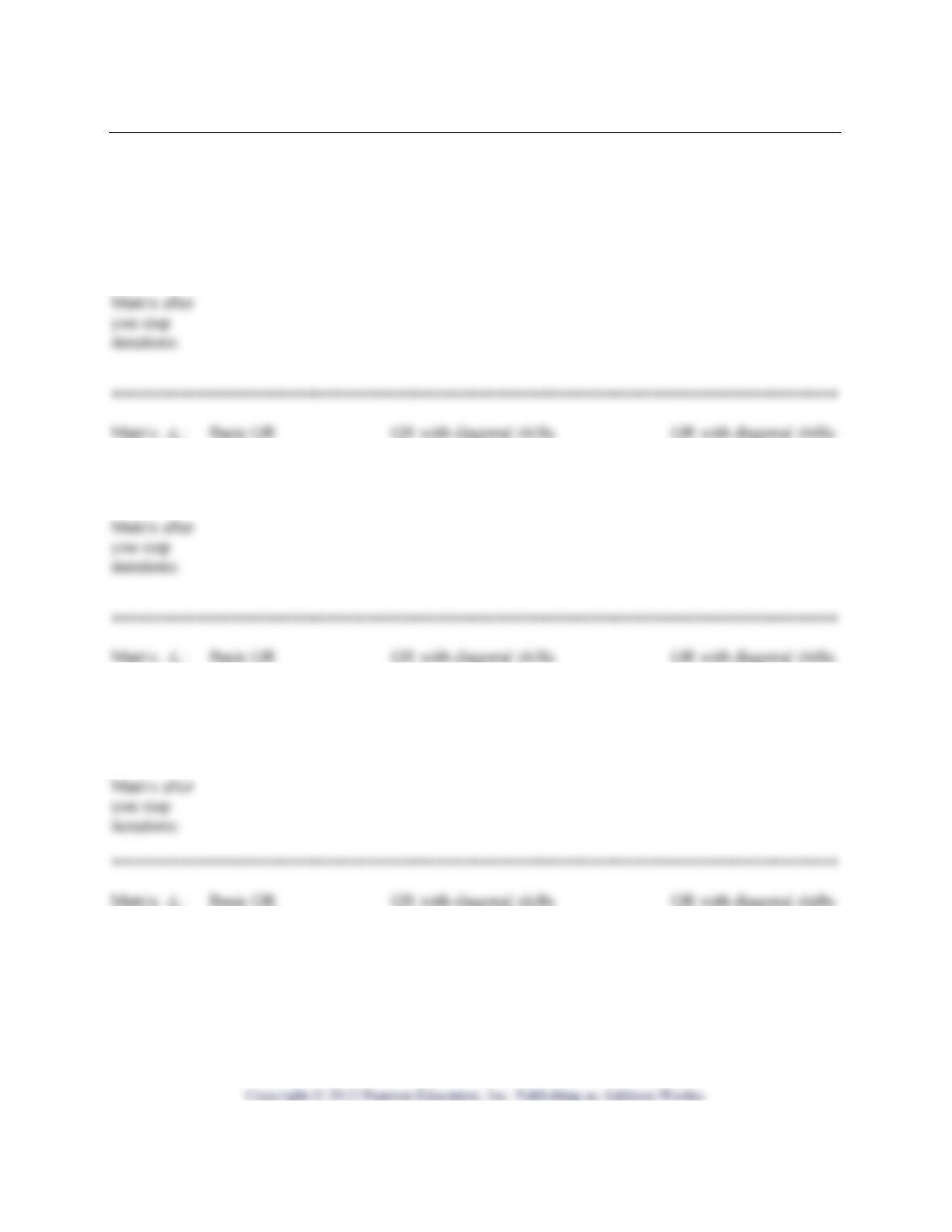
Results from Question 3
Matrix 3
A: Basic QR QR with diagonal shifts QR with diagonal shifts
tol = 0.001 tol = 0.001 tol = 0.0001
# steps _____ time =_____ # steps _____ time _____ # steps _____ time _____
tol = 0.001 tol = 0.001 tol = 0.0001
# steps _____ time =_____ # steps _____ time _____ # steps _____ time _____
tol = 0.001 tol = 0.001 tol = 0.0001
# steps _____ time =_____ # steps _____ time _____ # steps _____ time _____
tol = 0.001 tol = 0.001 tol = 0.0001
# steps _____ time =_____ # steps _____ time _____ # steps _____ time _____
Matrix after
you stop
iterations:
Page 5 of 6 MATLAB Project: QR Method for Calculating Eigenvalues
Note. To better understand the algorithms, the following commands will accomplish the basic QR method
used in question 3 for an nn×matrix A. First, type in the matrix A.
B = A; bound = 0.001; p = 0; num = 200;
while max(max(abs(tril(B,-1))))>bound %test size of entries in lower triangle
[Q R] = qr(B); B = R*Q;
p = p+1;
The following lines will accomplish the shift-deflate algorithm used in question 5, for an nn×matrix A.
B = A; bound = 0.001; p = 0; num = 20; [m,n]=size(A);
for i = n:-1:2 % work from row n to row 2
B = B(1:i,1:i); % deflate
while max(max((abs((B(i,1:i-1)))))> bound %test size of entries
Remarks about convergence. There is an excellent discussion of the theory of the QR method in
Understanding the QR Algorithm, by D. Watkins, SIAM Review 24 (1982), pp. 427-440. This paper
explains the geometric meaning of the algorithm and how it is an extension of the power method. (The
power method is presented in Section 5.8 in Lay’s text.) Briefly, the following things are true about the
QR method, for an nn×real matrix A.
(b) The matrices used above in this project were chosen so they have only real eigenvalues.
However, a general real matrix can have nonreal eigenvalues. In this case, the algorithm described above,
which uses only real QR factorizations, cannot possibly converge to an upper triangular matrix (why?).
Page 6 of 6 MATLAB Project: QR Method for Calculating Eigenvalues
For example, the following matrices have some complex eigenvalues:
010
001
100
⎡
⎤
⎢
⎥
⎢
⎥
⎢
⎥
⎣
⎦
and
0100
0010
0001
1000
⎡⎤
⎢⎥
⎢⎥
⎢⎥
⎢⎥
⎣⎦
.
Store the first matrix as A. Calculate eig(A) to see what its eigenvalues are. Type [Q R] = qr(A),
A = R*Q and repeat this command several times. You will see cycling. Then apply the basic method to
A – I. To do that, type qrbasic(A + eye(3),.0001). Now you will see convergence to a block
upper triangular matrix with 11×and 22× blocks as described above. Subtract I from this limit matrix.
Solve the characteristic equation for the 22× block, and verify that this gives two complex numbers.
These will be the nonreal eigenvalues of A, and the 11×block contains the third, real, eigenvalue of A.
MATLAB Project: Least Squares Solutions and Curve Fitting Name________________________
Purpose: To practice using the theory of Least Squares by calculating and plotting the Least
Squares line, quadratic curve, and cubic curve for two sets of experimental data
Prerequisite: Section 6.6
MATLAB functions used: inv, ones, norm, size, plot, hold, print, polyval, polyfit,
axis; and lsqdat from Laydata4 Toolbox
Define
11
22
1
1
1
k
k
k
nn
xx
xx
xx
X
⎡⎤
⎢⎥
⎢⎥
=⎢⎥
⎢⎥
⎣⎦
,
1
0
k
β
β
β
⎡⎤
⎢⎥
⎢⎥
=⎢⎥
⎢⎥
⎣⎦
β
and
1
n
y
y
⎡
⎤
⎢
⎥
=
⎢
⎥
⎢
⎥
⎣
⎦
y.
So
X
and y are known, and the entries of β are the unknowns. The system of equations X=βyis usually
inconsistent, but one can find an approximate solution by the Least Squares method. The Least Squares
solution will be a “best solution” in the sense that it produces a vector β for which the vector
X
−yβhas
smallest possible length. The length of
X
−yβ is called the Least Squares error.
In this project you will work with two different sets of experimental data. For each set of data,
you will calculate the Least Squares equations of degree 1, 2 and 3 and the error for each, and you will
1. Type [x0 y0] to see the vectors side by side, and examine this to familiarize yourself with the data.
Then type the following line to plot the 13 data points with * symbols, to establish scaling for the graph,
and to hold this picture so future plots will appear on same axes:
(a) Find the coefficients 0
β
and 1
β
for the Least Squares line, 10
yx
ββ
=+
. To do this, click on
the Command screen and type the following lines. These commands use the formula in the text:
X1 = [x0 ones(13,1)]
is 57.9 1 02.6yx=− (after rounding).
Calculate the error for the Least Squares line by typing err1 = norm(y0–X1*b1) and
Page 2 of 4 MATLAB Project: Least Squares Solutions and Curve Fitting
To plot the line, use semicolons as shown because there are many numbers in x, X and y but these
vectors are of interest only for plotting:
Remark. Of course you need only two points in order to plot a line, but this vector z will be useful in (b)
and (c) where you do need a lot of closely spaced points in order to get smooth looking plots of curves.
(b) Find the coefficients 0
β
, 1
β
, and 2
β
for the Least Squares quadratic 2
210
yx x
βββ
=++
for
the data x0 and y0 and the associated Least Squares error. Since x0, y0 and X1 are still in your
workspace, you can do these things by typing the following commands:
X2 = [ x0.^2 X1 ] (x0.^2 causes each entry of the vector x0 to be squared)
b2 = inv( X2’ * X2 ) * X2’ * y0 (calculate the coefficients for the quadratic)
err2 = norm( y0 – X2 * b2 ) (calculate the Least Squares error for the quadratic)
Record the equation and the error in the first table below. Then plot the quadratic. Since Z1 is still in your
workspace, you can do this by typing the following lines:
β
β
β
β
After you are sure the new commands are correct, execute them. Suggestion: display the cubic curve
with a different color and symbol, say as a green dotted curve by typing plot( z, y, ‘g:’) .
Remark. Your new lines will be almost identical to those you used in (b). You can avoid some
retyping by pressing the up arrow key until you find the command you want; modify it if necessary and
then press [Enter] to execute it.
Page 3 of 4 MATLAB Project: Least Squares Solutions and Curve Fitting
Least Squares Polynomials for Question 1
Equation Least Squares Error
Line
——————————————————————————–———————————————–
Quadratic
——————————————————————————–———————————————–
Cubic
——————————————————————————–———————————————–
2. In this question, repeat the calculations of question 1, using the vectors vel and drag. This is data
from a wind tunnel experiment on a model of an F-16 airplane climbing at a constant 5angle. The data
was supplied by Aerolab, Laurel, MD.
Drag is the force opposing the forward motion of the plane. It depends on velocity and is parallel
to the earth’s surface. (In general drag also depends on a lift coefficient which varies with the angle of
attack, and on the area of the wing, but those are constant in this example.)
(a) To begin, type the following commands to inspect the data and plot the new data points:
Record your results in the table below, print your graph, label the curves, and attach.
Least Squares Polynomials for Question 2
Equation Least Squares Error
Line
——————————————————————————–———————————————–
Page 4 of 4 MATLAB Project: Least Squares Solutions and Curve Fitting
(b) It is true that one can use the laws of physics to derive a formula for drag. When the area of
the wing and the lift coefficient are constant, this formula will be a polynomial
3. There are special functions in MATLAB for calculating Least Squares (LSQ) solutions, which are
much easier to use than the calculations you did above, and they give more accurate results when you
have large amounts of data. These functions are polyfit and polyval , and professionals use them
so you should know about them.
b = polyfit(x0,y0,k) (then b will be the row vector
[
]
10k
βββ
… )
(a) To evaluate the polynomial at chosen values, type
(b) Then you can type plot(z,y)to see the graph of the polynomial. For example, try the
following commands for yourself, and observe they give the same results as you got in question 2(c):