Page 2 of 3 MATLAB Project: Reduced Echelon Form and ref
2. Let B =
⎥
⎥
⎥
⎦
⎤
⎢
⎢
⎢
⎣
⎡−
7.65.00
7.02.03.0
21.01.0
.
(a) (hand) Calculate the reduced echelon form of B. Please show all steps. Hint: do all scaling at the end.
Remarks For the majority of small matrices like those used in linear algebra courses, ref will
return a very accurate result as it does in the two examples above. One of the reasons ref is accurate is
that it does not pivot on a position where the value is extremely small. Such a number is often inaccurate
in many digits as a result of roundoff error during previous row operations, and it is even possible that
theoretically it ought to be a true zero. The usual algorithm for Gaussian elimination chooses the next
pivot by looking “to the right and down” for the first nonzero entry in the first nonzero column. If that
entry happens to be a very inaccurate number, pivoting on it can lead to a very wrong final result.
3. (MATLAB) Use the same matrix B as in question 2. Here you will force ref(B)to return the wrong
answer by making the value of tol too small, and you will experiment to figure out a good estimate for
what is the default value of tol.
(a) Type each of the following commands and record the result:
ref(B, 1e-15)
ref(B, 1e-16)
Now you can be certain that the default value for tol is smaller than 10-15 but not smaller than 10-16.
Explain why:
MATLAB Project: Rank and Linear Independence Name________________________
Purpose: To define rank and learn its connection with linear independence
Prerequisite: Section 1.7
MATLAB functions used: ‘, rank; and indat, randomint, and ref from Laydata4 Toolbox
Definition. The rank of a matrix A is defined to be the number of pivot columns in A. Notice this is well
defined since the reduced echelon form of a matrix is unique.
Example 1. Let A =
12 3 4
45 6 7
691215
11 1 1
⎡⎤
⎢⎥
⎢⎥
⎢⎥
⎢⎥
⎣⎦
. Type A, ref(A)to see A and ans =
10 12
01 2 3
00 0 0
00 0 0
−
⎡⎤
⎢⎥
⎢⎥
⎢⎥
⎢⎥
⎣⎦
.
There are two pivot columns in the reduced matrix so the rank of A is 2. Type rank(A)to see ans=2.
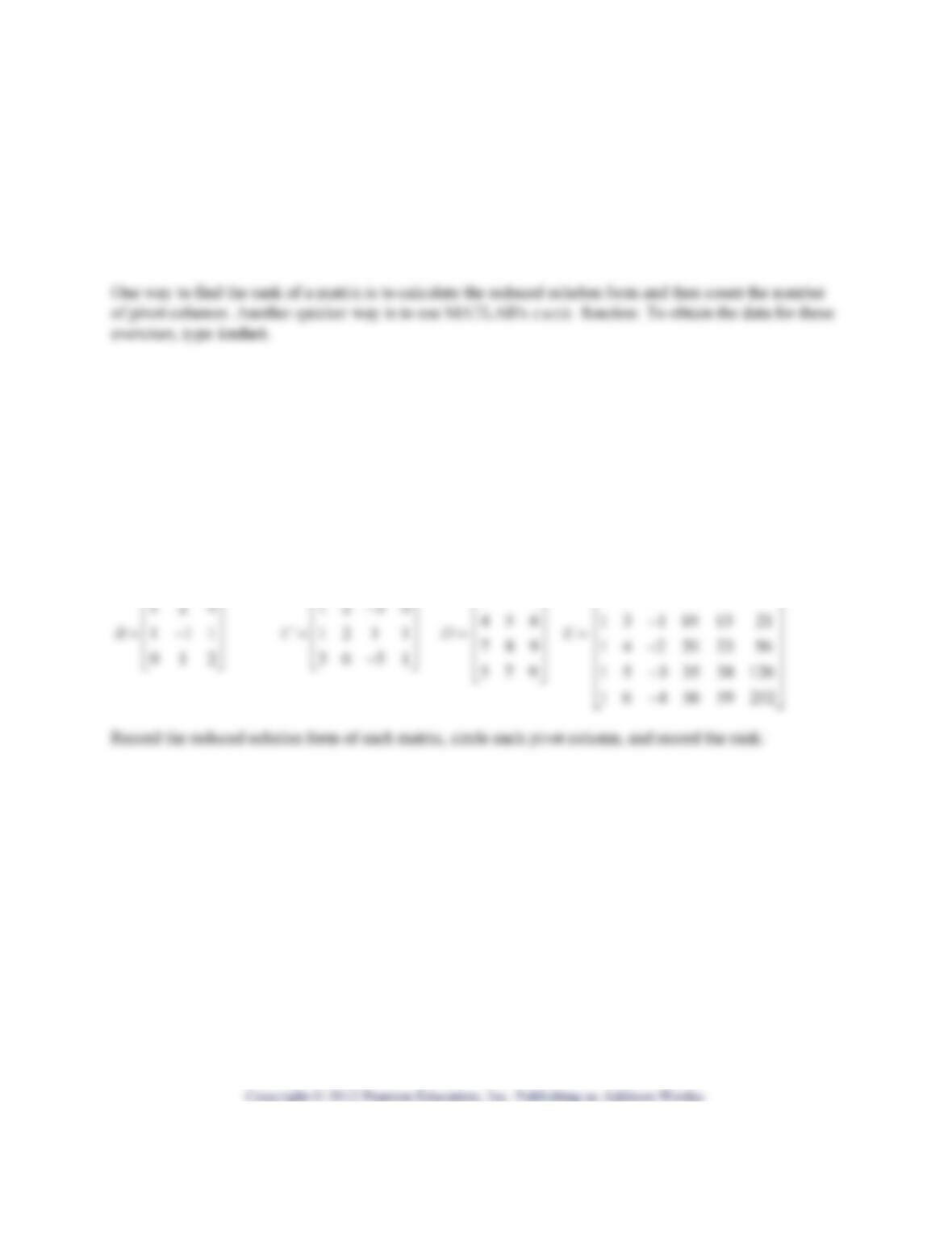
1. Use both of the above methods to find the rank of each of the following four matrices. For example,
type B, ref(B), rank(B)and fill in the blanks below.
⎢
⎢
⎢
⎢
⎣
⎢
⎢
⎢
⎢
⎢
⎢
⎢
⎣
123
⎡
⎤
11 1 1 4 1
12 0 4 7 6
⎡
⎤
⎢
⎥
Rank: _________ _________ _________ ____________
Page 2 of 3 MATLAB Project: Rank and Linear Independence
2. (hand) Read the definition of linear independence in Section 1.7. Let
[
]
12 k
M=vv v…be a
3. (MATLAB) Use the method of question 2 to answer the questions below. In each case, write the
appropriate matrix, use MATLAB to calculate its rank, and record the rank. To learn how to store a
matrix, see Section 1 of the computer project “Getting Started with MATLAB” or Lay’s Study Guide.
Example 2. The set
1234
2345
,,,
3456
0111
⎧⎫
⎡⎤⎡⎤⎡⎤⎡⎤
⎪⎪
⎢⎥⎢⎥⎢⎥⎢⎥
⎪⎪
⎢⎥⎢⎥⎢⎥⎢⎥
⎨⎬
⎢⎥⎢⎥⎢⎥⎢⎥
⎪⎪
⎢⎥⎢⎥⎢⎥⎢⎥
⎪⎪
⎣⎦⎣⎦⎣⎦⎣⎦
⎩⎭
is not linearly independent. Verify this by typing F,ref(F).
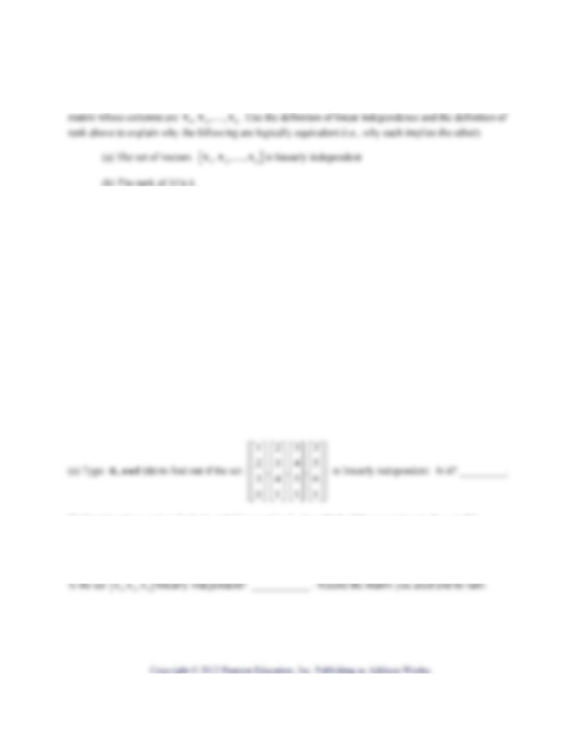
(b) Examine the matrices B, C, D, and E in question 1. For which of these matrices is the set of its
columns a linearly independent set?
_____________________.
(c) Let
[
]
12351=v,
[
]
211 2 9=−v, and
[
]
33400=v.
4. (MATLAB and hand) The transpose of a matrix
X
is defined to be the matrix T
Xwhose columns are
formed from the corresponding rows of
X
. For example, if 123
456
X
⎡
⎤
=
⎢
⎥
⎣
⎦, then
14
25
36
T
X
⎡⎤
⎢⎥
=⎢⎥
⎢⎥
⎣⎦
.
We want to determine how the rank of a matrix compares with the rank of its transpose. In MATLAB, the
single quote creates transpose — for example, typing A’ will create the transpose of A. Do at least 20
experiments to compare the rank of a matrix with the rank of its transpose. Use matrices of many different
sizes.
MATLAB Project: Visualizing Linear Transformations of the Plane Name___________________
Purpose: To understand the standard matrix of a linear transformation
Prerequisite: Section 1.8 and 1.9
MATLAB functions used: visdat and drawpoly from Laydata4 Toolbox
Background. As shown in Theorem 10 in Section 1.9, when a linear transformation :nn
T→is
given, it can be identified with a matrix, and there is an easy way to get a formula for the function as
follows. Let : nn
T→be a linear transformation and let 12
,,,
n
ee e…denote the columns of the nn×
1. Example. The 22×linear transformation that maps e1 to e1 + e2 and e2 to e1 – e2 is 11
11
⎡⎤
⎢⎥
−
⎣⎦
.
The 33×matrix transformation that maps e1 to
3
2
1
⎡
⎤
⎢
⎥
−
⎢
⎥
⎢
⎥
⎣
⎦
, e2 to
6
0
7
⎡
⎤
⎢
⎥
⎢
⎥
⎢
⎥
⎣
⎦
and e3 to
5
4
1
⎡
⎤
⎢
⎥
⎢
⎥
⎢
⎥
−
⎣
⎦
is
36 5
20 4
17 1
⎡⎤
⎢⎥
−
⎢⎥
⎢⎥
−
⎣⎦
.
2. Example. The function that reflects 2
across the line yx=− is a linear transformation. It must map
3. Exercise. (hand) (a) Write a 22×matrix that maps e1 to 4e2 and e2 to –e1 :
(b) Write a 22×matrix that reflects 2
across the line yx=:
4. Exercise. (hand) Let 10
11
M⎡⎤
=⎢⎥
⎣⎦
.
(a) Explain why the function ( )TM=
xxmaps the x-axis onto the line yx=, and why it maps the line
Page 2 of 8 MATLAB Project: Visualizing Linear Transformations of the Plane
(b) Sketch here what you showed algebraically in 4(a). That is, sketch the x-axis and the line 2y= on the
left axes below, and sketch and label their images on the right:
Still more background. Because a matrix transformation maps parallel lines to parallel lines, it will map
any parallelogram to another parallelogram. (The parallelogram could be degenerate—one line segment
or a single point.) When a linear transformation and parallelogram are given, the easy way to draw the
image of the parallelogram is to plot the images of its four vertices and connect those points to make a
parallelogram.
Define the standard unit square to be the square in 2
whose vertices are (0,0), (1,0), (1,1) and
(0,1). When you want to visualize what a 22×matrix transformation does geometrically, it is
particularly useful to sketch the image of this standard square. Seeing how this square gets moved or
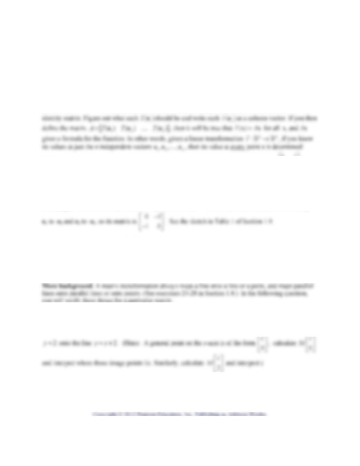
Example. Continue to use ( )TM=xxwhere 10
11
M
⎡
⎤
=
⎢
⎥
⎣
⎦. Sketch the image of the standard unit square:
So you can see that the y-axis stays fixed and the x-axis is mapped onto the line yx=, causing a vertical
shear of the plane. See more examples like this in Table 3 in Section 1.9.
Example. Find a matrix M which maps the standard unit square to the parallelogram with vertices (0,0),
(3,1), (2,2), (-1,1). To do this, sketch the parallelogram and recognize that Me1 and Me2 must be (3,1) and
⎡
⎢
⎣
⎡
⎢
⎣
Page 3 of 8 MATLAB Project: Visualizing Linear Transformations of the Plane
Be sure you understand why these are the only two matrices that will work here. Calculate the image of
(1,1) under each of these matrices, to verify that it is the point (2,2).
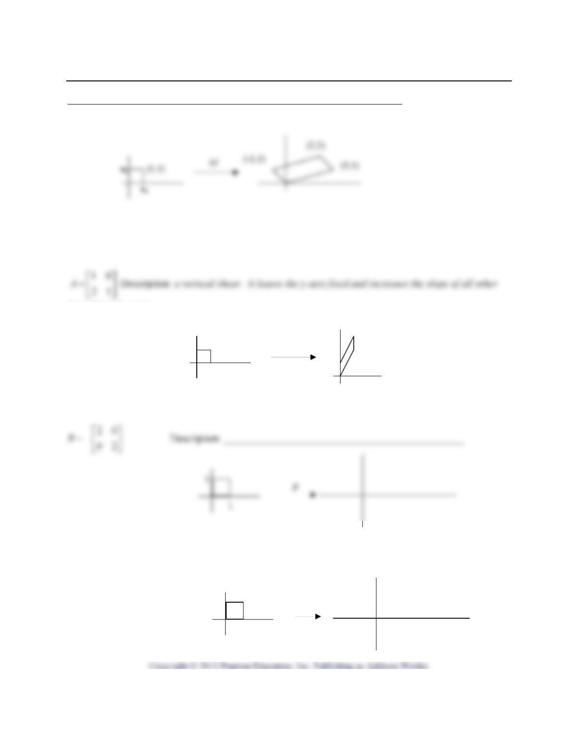
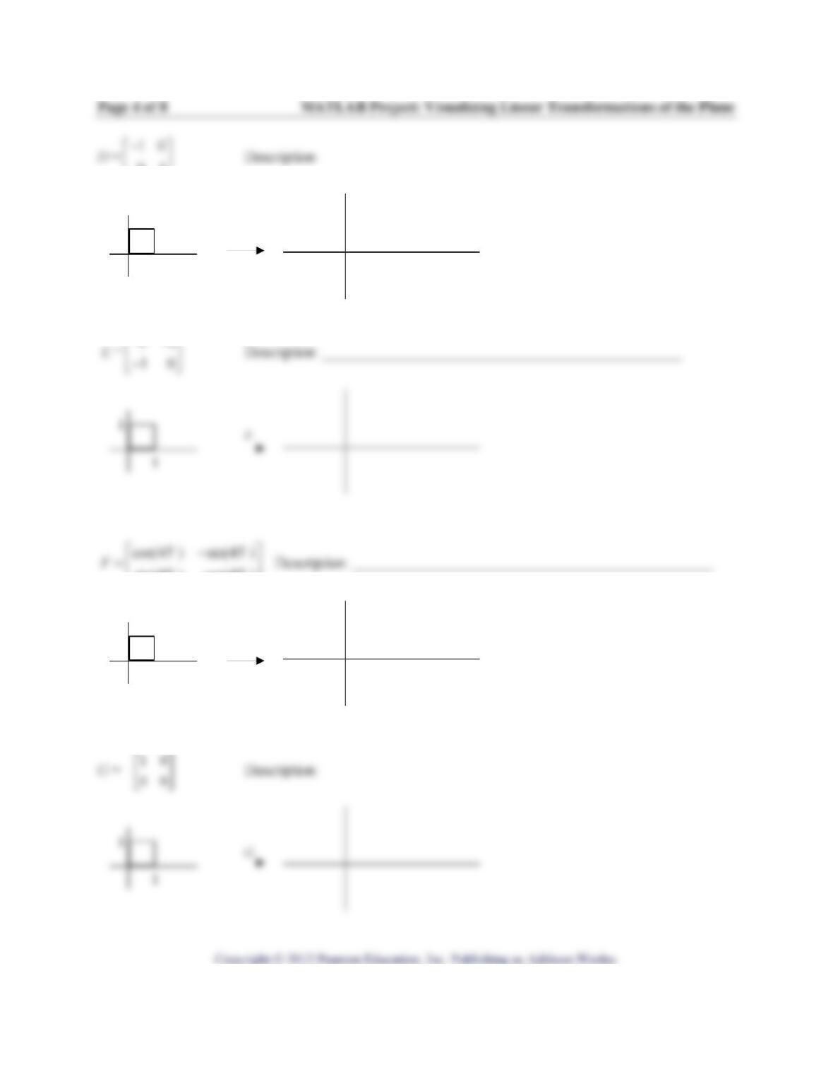
5. Exercise. (hand) Each of the seven matrices below is one of the special, simple types described in
Sections 1.8 and 1.9. Each determines a linear transformation of 2
. For each, sketch the image of the
standard unit square, label the vertices of the image, and describe how the matrix is transforming the
plane. To get you started, answers are given for the first matrix.
lines through origin.
(1,3)
1
1
A(1,2)
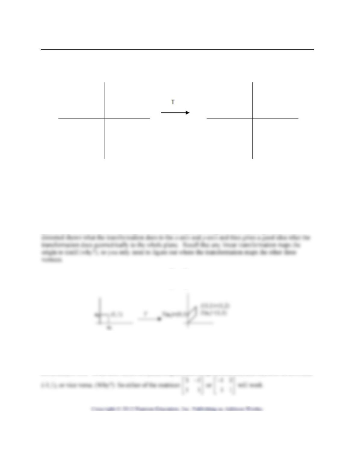
10
01
C⎡⎤
=⎢⎥
−
⎣⎦
Description: ________________________________________________
1
1
C
01
⎣⎦
1
1
D
E
sin(45 ) cos(45 )
⎣⎦
1
1
F
6. Exercise. (MATLAB) In computer graphics, transformations are usually accomplished by applying a
succession of simple matrix transformations—dilations, shears, reflections, rotations and projections.
Here you will do a variety of such.
To begin, type visdat to get the matrices A, B, …, G used above. You will also get a matrix
called box whose columns contain the coordinates of the vertices of the standard unit square.
(a) Type A, box and A*box and record these below. Notice the command A*box causes
MATLAB to multiply A times each column of box – i.e., the columns of A*box are the images under A
of the vertices of the standard unit square.
When X is a matrix with two rows, each column represents a point in 2
, and the command
drawpoly(X) will plot those points and draw a line segment from each to the next one. Try this: type
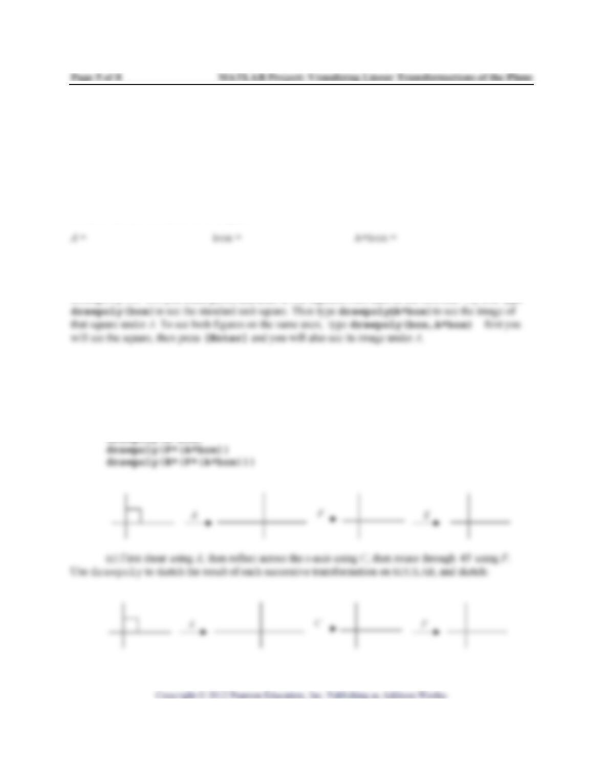
(b) The commands below perform several successive transformations of the standard unit square.
The first one does a shear using A. The second does the shear followed by rotation of the plane through
45using F. The third does the shear followed by the rotation and then reflects the plane across the line
yx=− using E. Type these lines, and watch carefully to see the result of each successive transformation.
Sketch the new figure obtained after each step:
drawpoly(A*box)
7. Exercise. (hand) Sketch the parallelogram with vertices (0,0), (4,2), (0,-4), (4,-2) and write two
different 22×matrices X and Y which would transform the standard unit square into this parallelogram.
Use drawpoly to verify that your matrices work:
8. Exercise. (hand) Sketch the parallelogram with vertices (1,1), (1,2), (3,1), (3,2). Explain why no 22×
matrix transformation could map the standard unit square onto this figure.
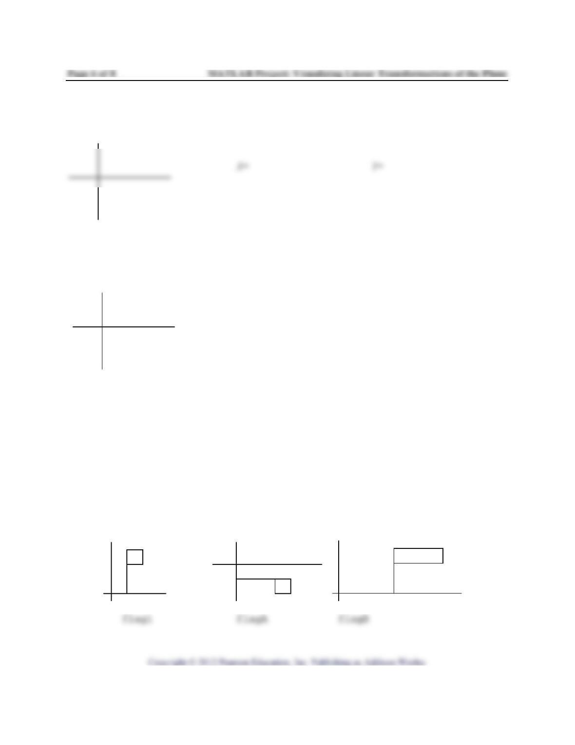
Example. In the figure below called flag1, the flagpole is from (1,0) to (1,3), and the vertices of the
flag itself are (1,2), (1,3), (2,3), and (2,2). Label these points. We will find matrices which transform
flag1 into the other figures, flagA and flagB.
Page 7 of 8 MATLAB Project: Visualizing Linear Transformations of the Plane
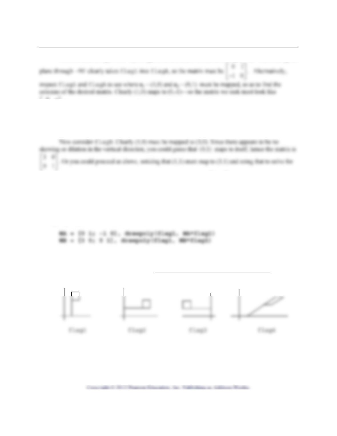
First consider flagA. One way to figure out the matrix would be to simply “see” that rotating the
⎡
⎢
⎣
0
1
a
b
⎡⎤
⎢⎥
−
⎣⎦
. It is also easy to see by inspection that (1,1) must map to (1,-1), so solve the equation
011
111
a
b
⎡⎤⎡⎤⎡⎤
=
⎢⎥⎢⎥⎢⎥
−−
⎣⎦⎣⎦⎣⎦
for a and b, and you will find this yields the same matrix 01
10
⎡
⎤
⎢
⎥
−
⎣
⎦.
the entries of the second column of the matrix. This would also yield 30
01
⎡
⎤
⎢
⎥
⎣
⎦.
Whatever method you use to calculate the matrix, you should check that your matrix really does
what you want. An easy way would be to use drawpoly to sketch flag1 and its image under A. The
vertices of flag1 are already stored in the matrix flag1, so store your matrices and then use
drawpoly. Try these commands to do that:
9. Exercise. The figure flag1 is shown again below. One at a time, consider each of the other three
flags sketched below and find a 22×matrix which maps flag1 onto it. Use drawpoly to verify that
each of your matrices does what you want, and record each matrix below the appropriate figure.
Matrices: _______________ _______________ _______________ ___________________
10. Exercise. (Extra credit) Let : nn
T→be a linear transformation. As pointed out in “Background”
on page 1, T is completely determined by its values on the special vectors 12
,,,
n
ee e….
Prove that T is completely determined by its values on any n linearly independent vectors.
Here is an outline of the proof to get you started. Assume : nn
T→is a linear transformation. Let
MATLAB Project: Population Migration Name_______________________________
Purpose: To study the population movement described in Exercise 11, Section 1.10 in more detail
Prerequisite: Section 1.10
When you are finished, attach your plots and turn in with these pages.
1. Read Exercise 11, Sec. 1.10. Notice this is a simple migration model, which assumes people just
move around and the total population of the US remains constant. Hence, if x is a vector whose
components are the number of people in each area this year, then
M
xis the number in each area next year.
(a) To obtain the data from Laydata4 Toolbox for this exercise, type the lines
c1s10
11
(b) (hand) Describe the calculations needed to produce the entries in M, based on the information
in the text.
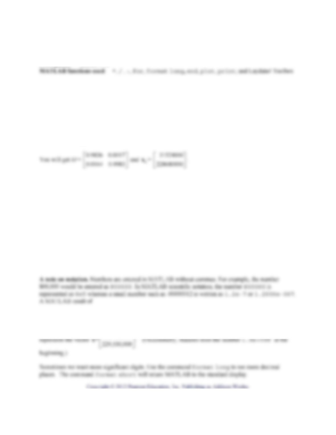
>>x=1.0e+008 *
0.3067
2.2953
⎡⎤
2. Continue to consider the migration model in Exercise 11, Section 1.10.
(a) Calculate the population in Californian (CA) and in the rest of the United States (US) for the
years 1990 – 2000 and store that data as the columns of a matrix P.
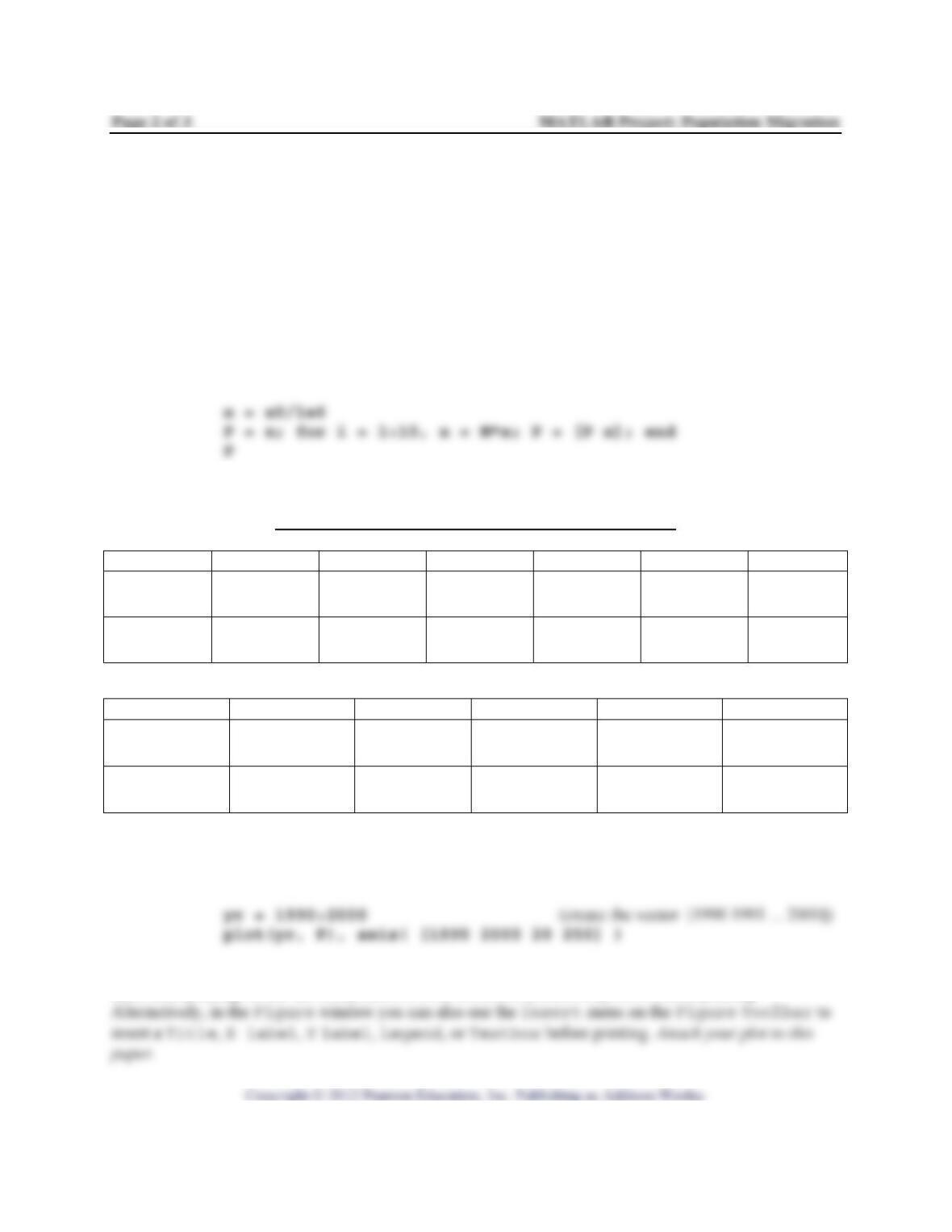
To do this, type the lines below. The first line converts the population data to millions. The
second line builds P one column at a time using a for loop. The loop “for i = 1:10 … end”
causes MATLAB to perform the commands x = M*x; P = [P x]; ten times. Each iteration
calculates a new x and adjoins that new column to the columns already in P. To learn more about for
loops in MATLAB, type help for or see the MATLAB boxes in the Study Guide. The semicolons are
used to suppress printing during the calculations. The third line causes P to be displayed after the
calculations are finished.
Record the data from P in the table below. Round each number to 4 digits.
Population in millions, assuming no external migration
Year 1990 1991 1992 1993 1994 1995
CA
Rest of US
Year 1996 1997 1998 1999 2000
CA
Rest of US
(b) Plot the population in CA, and the population in the rest of the US, versus years, on the same
graph. The following lines will do this:
(c) Print your graph, title it, and label each curve “CA” and “US.” You can do the labeling by
hand after printing, or use the commands title, xlabel, ylabel, gtext before printing.

3. Suppose instead that the population is actually increasing each year because of immigration from
outside the U.S., say 0.1 million people immigrate to CA and 2 million to the rest of the US each year.
Then if data is expressed in millions and x is the population vector this year, .1
2
M⎡⎤
+⎢⎥
⎣⎦
xwill be the
population vector next year.
(a) Calculate the new population predictions for 1990-2000; the following lines will do this:
Record the data from P in the following table. Round each number to 4 or 5 digits.
Population in millions, assuming external migration
Year 1990 1991 1992 1993 1994 1995
CA
Rest of US
Year 1996 1997 1998 1999 2000
CA
Rest of US
(b) Arrow up to execute the plot command you typed before. This will produce a graph of the
new data. Print and label this graph as instructed above, and attach to this paper.
MATLAB Project: Elementary Analysis of the Spotted Owl Population Name_________________
Purpose: To study the owl population with several different survival rates for juveniles
Prerequisite: Section 1.10 and the example at the beginning of Chapter 5
MATLAB functions used: +, * , ‘ , :, sum, for, end, plot, print; and owldat from Laydata4
Toolbox
of owls in each stage in year k, t is the survival rate for juvenile →subadult, and 1kk
A
+=xx
. The
example in the text reports that the population will eventually die out if t = .18 but not if t = .30. You will
verify these facts here.
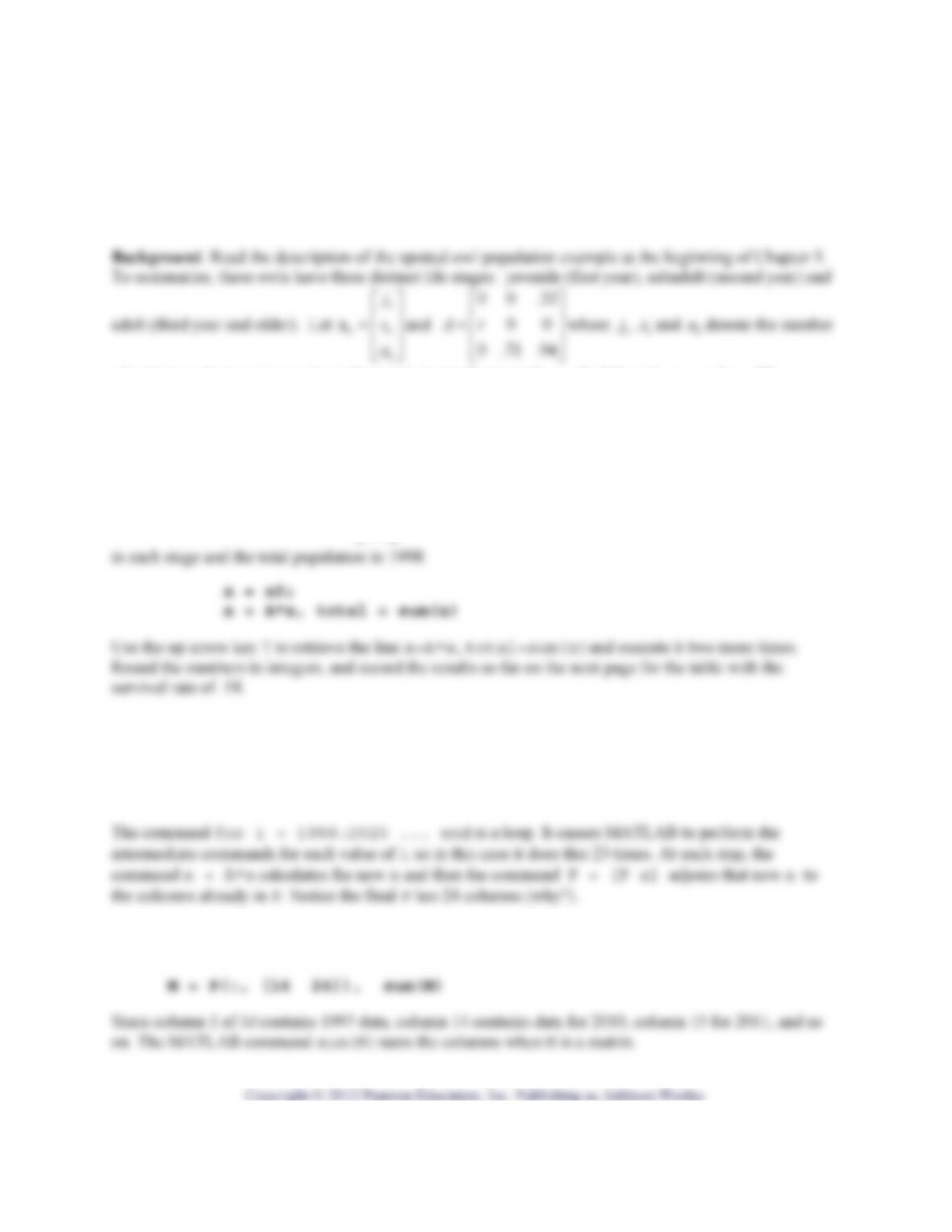
1. Let t = .18 and suppose there are 100 owls in each life stage in 1997. Type owldat to get the matrix
A (with t = .18) and the vector 0
100
100
100
⎡⎤
⎢⎥
=⎢⎥
⎢⎥
⎣⎦
x. Use the following MATLAB code to calculate the population
2. (a) It is tedious to do the calculation year by year, as in question 1. Type the following line to calculate
the population vectors through year 2020 and store these as the columns of a matrix P.
x=x0; P=x; for i = 1998:2020, x=A*x; P = [P x]; end
P
Record the data for 2010, 2020 in the table with the survival rate of .18 on the next page, and round the
numbers to integers. An easy way to determine this data is to enter:
Page 2 of 3 MATLAB Project: Elementary Analysis of the Spotted Owl Population
Population when the juvenile→subadult survival rate is .18
Year 1997 1998 1999 2000 2010 2020
Juvenile 100
Subadult 100
Adult 100
Total 300
(b) Type the following line to plot curves for the data in each of the three age groups.
(c) Insert a Textbox for each curve by using the pulldown Insert menu on the Figure Toolbar.
Label your curves (“Adult,” “Subadult,” “Juvenile”). Another option is to label the curves by hand
after printing them out.
(d) Does it appear that the owls will die out if the survival rate is t=.18? ___________________

3. Now let t = .30 and repeat the instructions of question 2 to verify that the population of owls will not
die out if the survival rate of juveniles to subadults is .30 instead of .18. To begin, type A(2,1)=.30
and then use the arrow up key ↑ to retrieve the line with the for loop, so you do not have to type it again.
Population when the juvenile→subadult survival rate is .30
Year 1997 1998 1999 2000 2010 2020
Juvenile 100
Subadult 100
Adult 100
Total 300
4. Repeat the calculations and plotting in question 3 for these additional values of t: .20, .24, .26, .28.
You do not have to record the data or print graphs for these, but just list all the values of t for which your
MATLAB Project: Lower Triangular Matrices Name_______________________________
Purpose: To investigate properties of products of lower triangular matrices
Prerequisite: Section 2.1
MATLAB functions used: + , * , tril, rand, eye
1. Create several lower triangular nn×matrices, calculate their products in pairs, and see what appears to
be true. For example you could do this for two different 22×matrices whose lower triangle entries are
random numbers by typing:
n = 2
L1 = tril(rand(n)), L2 = tril(rand(n)), L1*L2, L2*L1
Execute the second line several times and inspect the result each time. Repeat with n = 3,4,5. The easy
way is to press the up arrow ↑ on your keyboard to retrieve the second line, and then press [Enter] to
execute it again.
(b) Try the following calculation several times A=rand(2),B=rand(2),A*B,B*A. Does your
conjecture in part (a) appear to be true for non-triangular matrices?