
4. Consider the sketch below. The standard unit square is shown on the left.
(a) (hand) Find 33×matrices A, B and C so that applying your new matrices in succession to
homogeneous coordinates of that square will successively transform it as shown. Write in each of
your matrices:
A= B= C=
(b) (MATLAB) Store your new matrices A, B and C and type M = C*B*A to calculate the product
M = CBA. This is the composition of the three functions you created. Record it.
M =
MATLAB Project: Subspaces Name_______________________________
Purpose: To understand what is required for two subspaces of n
\with the same dimension to be
the same set
Prerequisite: Section 4.6 or 2.9
MATLAB functions used: rank, diary; and ref and submats from Laydata4 Toolbox
Remarks. Your instructor will supply a pair of matrices A and B, each having five rows. There are such
pairs in the file submats, and you may be assigned one of those.
Question 1 is easy, but you will need to think how to answer question 2. Discuss it with each other —
this can really help. Once you figure out a method it will not take long to do the calculations. Observe that
Col A and Col B are obviously subspaces of 5
\.
Directions. Use the matrices A and B which your instructor supplies. Employ MATLAB to do whatever
1. Verify that Col A and Col B have the same dimension.
2. Determine whether or not Col A and Col B are the same subspace of 5
\. Explain what you
calculated and why it worked.
Notice this is not obvious. For example, if two subspaces of 3
\each have dimension 1, each will
be a line through the origin, but they might not be the same line. If each has dimension 2, they are planes
MATLAB Project: Markov Chains and Long Range Predictions Name____________________
Purpose: To analyze several Markov chains and investigate steady state vectors
Prerequisite: Section 4.9
MATLAB functions used: *, ^ , – , / , eye, sum ; markdat and ref from Laydata4 Toolbox
Background. Read Section 4.9 in the text, about Markov chains.
1. Read Exercises 2 and 12 in Section 4.9. They concern a Markov chain with the system matrix P shown
below. In these exercises there are three foods and the ,ij
entry of P is the probability that if an animal
chooses food j on the first trial, then it will choose food i on the second trial. Therefore the ,ij
entry of
2
P
is the probability that if an animal chooses food
j
on the first trial, it will choose food i on the third
trial.
(a) Type markdat to get the data for this project. The matrix for exercises 2 and 12 is called P and
is shown below. Type P^2 to calculate 2
P
and record:
P
(b) (hand) Suppose an animal chooses food #1 on the first trial. Use Pand 2
P
to answer the
following. Find the probability the animal will:
Choose food #2 on the second trial: _________________
Choose food #2 on the third trial: ___________________
Choose food #3 on the third trial: ___________________
2. Read Exercise 4 in Section 4.9 and solve it as follows.
(a) Write the matrix W and the initial vector v describing weather “today” in Exercise 4. Be careful!
The matrix W should be stochastic, and v should be a probability vector.
W = v =
(b) (MATLAB) Store your vector v as a column and type W*v to calculate Wv.
Record Wv=
(c) Now store the new initial vector for Monday, v=qand type (W^2)*v.
Record 2
Wv=
Using this, what is the chance of good weather on Wednesday? _____________
(d) Calculate the steady state vector q for W using the method shown in question 1(c) above.
In the long run, what is the probability the weather will be good on a given day? ________________
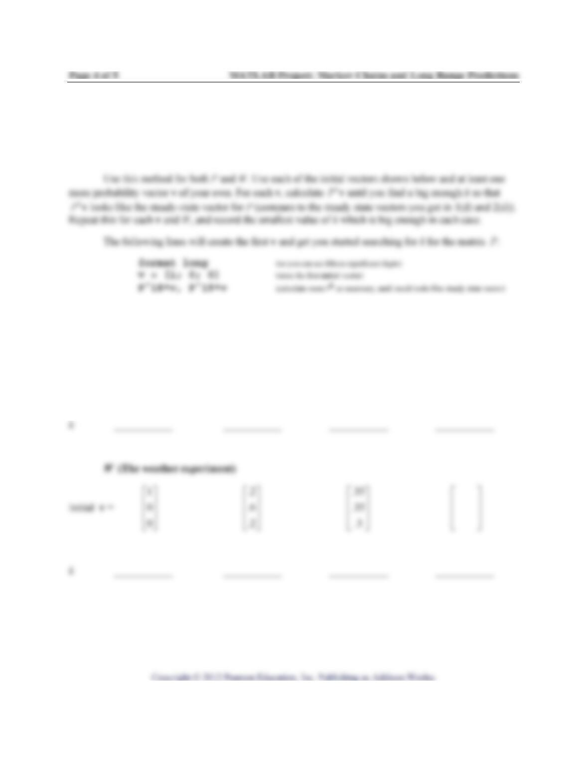
3. According to Theorem 18, when P is stochastic and regular, and v is any probability vector, the
sequence of vectors v,
P
v,2
Pv, … will converge, and the limit vector will be the steady-state vector of
P. In other words, when the power k is big enough, k
Pvwill look like the unique steady-state vector.
This method is not an efficient way to calculate the steady-state vector, but it is interesting to see
sequences v,
P
v,2
Pv, … converge for a few examples.
P (The animal experiment)
Initial v =
1
0
0
⎡⎤
⎢⎥
⎢⎥
⎢⎥
⎣⎦
.2
.6
.2
⎡
⎤
⎢
⎥
⎢
⎥
⎢
⎥
⎣
⎦
.35
.35
.3
⎡
⎤
⎢
⎥
⎢
⎥
⎢
⎥
⎣
⎦
⎡⎤
⎢⎥
⎢⎥
⎢⎥
⎣⎦
⎡
⎢
⎢
⎢
⎣
⎡
⎢
⎢
⎢
⎣

Page 5 of 5 MATLAB Project: Markov Chains and Long Range Predictions
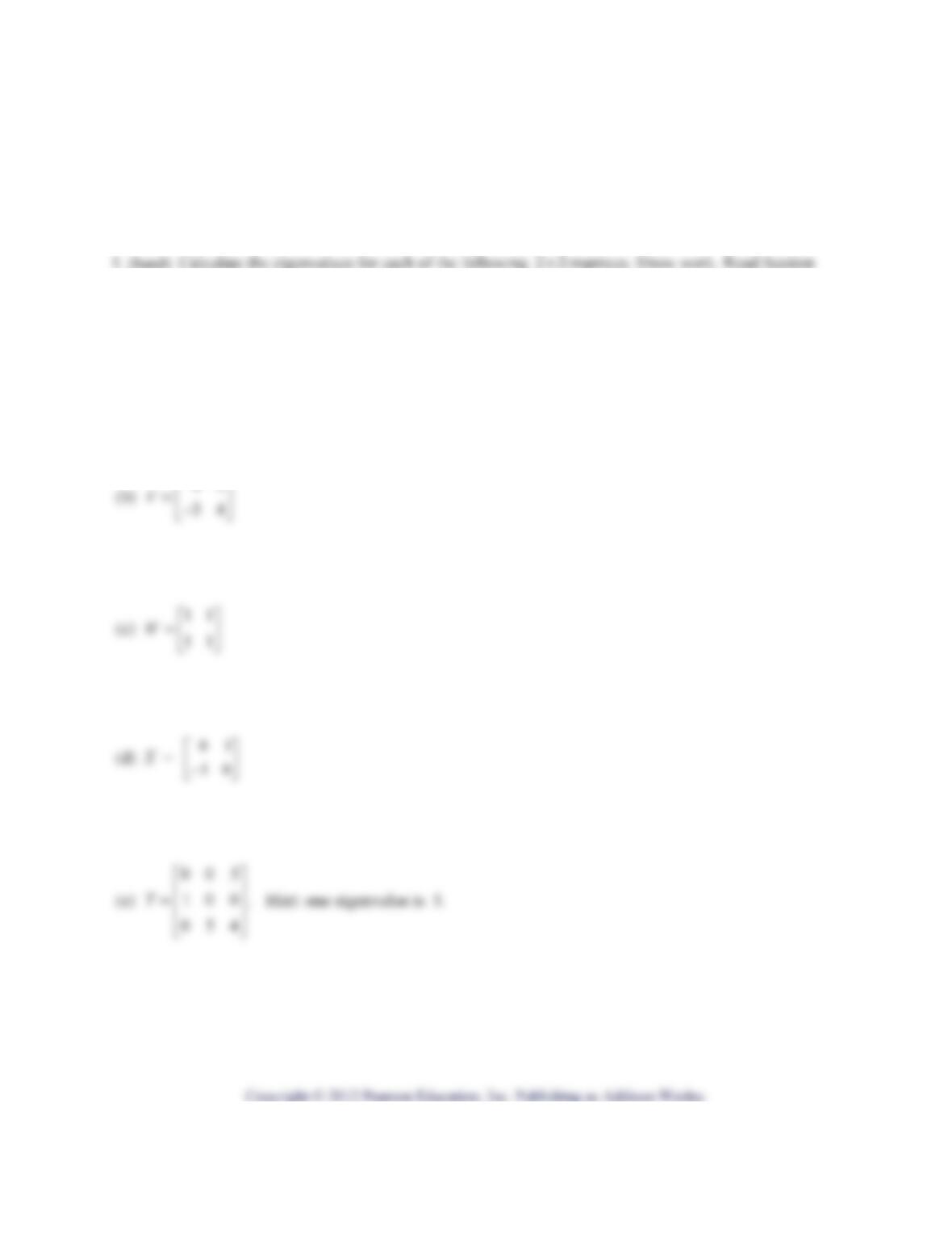
4. Consider the following matrices: 1
.7 .2 .6
0.2.4
.3 .6 0
P
⎡
⎤
⎢
⎥
=
⎢
⎥
⎢
⎥
⎣
⎦
, 2
.7 .2 .6
0.20
.3 .6 .4
P
⎡
⎤
⎢
⎥
=
⎢
⎥
⎢
⎥
⎣
⎦
, 3
010
100
001
P
⎡⎤
⎢⎥
=⎢⎥
⎢⎥
⎣⎦
.
(b) Type format to restore MATLAB’s usual short form for display of numbers. Then calculate steady
state vectors for 1
P,2
P, and 3
P using the method in question 1(c) above. The matrices will be called P1,
P2 and P3 in your workspace. Record the steady state vectors in the table below. Use Theorem 18 or
some calculations to decide whether the steady state vector is unique.
Steady state vector
Is the steady
state
vector unique?
If v =
1
0
0
⎡
⎤
⎢
⎥
⎢
⎥
⎣
⎦
, does k
Pvconverge as k gets large?
If not, what does happen?
MATLAB Project: Real and Complex Eigenvalues Name_______________________________
Purpose: To see examples of nonreal eigenvalues, and to learn how to use MATLAB’s eig
function operations
Prerequisite: Section 5.5
MATLAB functions used: eig, *; and cxeigdat from Laydata4 Toolbox
5.5 in the text for examples.
(a) 52
43
U⎡⎤
=⎢⎥
⎣⎦
2. (hand) Create some new examples. For each of the 22×matrices U, V, W, and X, it is easy to change
the sign of one entry so that the new matrix has nonreal eigenvalues if they were real before; or has real
3. (MATLAB) Type cxeigdat to get the matrices used in question 1. For each matrix A, use eig to get
a matrix D whose diagonal entries are the eigenvalues of A, and a matrix P whose columns are associated
eigenvectors. Record P and D, and inspect D to be sure the eigenvalues produced by eig agree with
what you calculated by hand in question 1. Study the proof of Theorem 5, Sec. 5.3 to understand why the
(a) 52
43
U⎡⎤
=⎢⎥
⎣⎦
P = D =
(b) 43
34
V⎡⎤
=⎢⎥
−
⎣⎦
P = D =
(c) 11
11
W⎡⎤
=⎢⎥
⎣⎦
P = D =
(d) X = ⎥
⎦
⎤
⎢
⎣
⎡
−01
10 P = D =
MATLAB Project: Using Eigenvalues to Study Spotted Owls Name_____________________
Purpose: To use eigenvalues and eigenvectors to understand the dynamics of this population and
determine experimentally the critical rate for survival of juveniles to subadults—the
value which that rate must equal or exceed for the population to survive
Prerequisite: Sections 5.5 and 5.6
MATLAB functions used: *, \ , :, sum, abs, for, eig, plot; and owldat from Laydata4 Toolbox
Background. The spotted owls have three distinct life stages: juvenile (first year), subadult (second year)
and adult (third year and older). Let
k
kk
k
j
s
a
⎡
⎤
⎢
⎥
=
⎢
⎥
⎢
⎥
⎣
⎦
xand
00.33
00
0.71.94
At
⎡
⎤
⎢
⎥
=
⎢
⎥
⎢
⎥
⎣
⎦
where k
j, k
s
, and k
adenote the
number of owls in each stage in year k and 1kk
A
+=xx
. As you may have seen in the earlier computer
To begin, type owldat to get the matrix for t = .18,
00.33
.18 0 0
0.71.94
A
⎡
⎤
⎢
⎥
=
⎢
⎥
⎢
⎥
⎣
⎦
. Then type the
following lines:
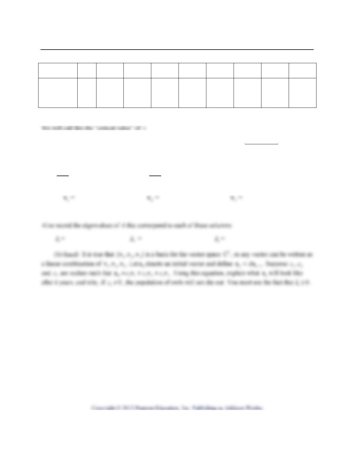
Page 2 of 5 MATLAB Project: Using Eigenvalues to Study Spotted Owls
Survival rate
juv→subadul
t
t = .18 .20 .22 .24 .25 .26 .28 .30
Dominant
eigenvalue
of A
λ
(b) Of the values you used for t, which is the smallest one for which 11
λ
≥? ___________________
2. Now assign A(2,1)the value that you just found which causes t to have the critical value. Thus, the
dominant eigenvalue 1
λ
of your matrix A will be slightly larger than 1.
(a) Type [V D] = eig(A). Notice that the dominant eigenvalue of A, which we want to call 1
λ
,
is the third diagonal entry of D, hence the third column of V is an eigenvector corresponding to 1
λ
. So
record the third column of V as 1
v and the first two columns of V as 2
v and 3
v.
Page 3 of 5 MATLAB Project: Using Eigenvalues to Study Spotted Owls
Remark: The space 3
^is much like 3
\. Its elements are all triples of complex numbers, and its scalars
are the complex numbers. Also, {(1,0,0), (0,1,0), (0,0,1)} is a basis for 3
^so its dimension is three;
hence, any three independent vectors in 3
^form a basis for the space. Finally, the vectors 123
,,vvv
found in question 2 are linearly independent. You can check that directly, or just notice that the three
eigenvalues of A are distinct.
(c) Let the initial vector be 0
100
100
100
⎡⎤
⎢⎥
=⎢⎥
⎢⎥
⎣⎦
x. Type the following lines to rearrange the columns of V so the
eigenvector corresponding to 1
λ
is the first column and then to solve 0112233
cc c=+ +xvvv
for the i
c’s:
3. Continue to use 0
100
100
100
⎡⎤
⎢⎥
=⎢⎥
⎢⎥
⎣⎦
xas the initial vector. Choose two values of t: 1
tshould be less than the
critical value you found above, and 2
t greater than that critical value. Record the values you choose:
1
t = __________ 2
t = __________
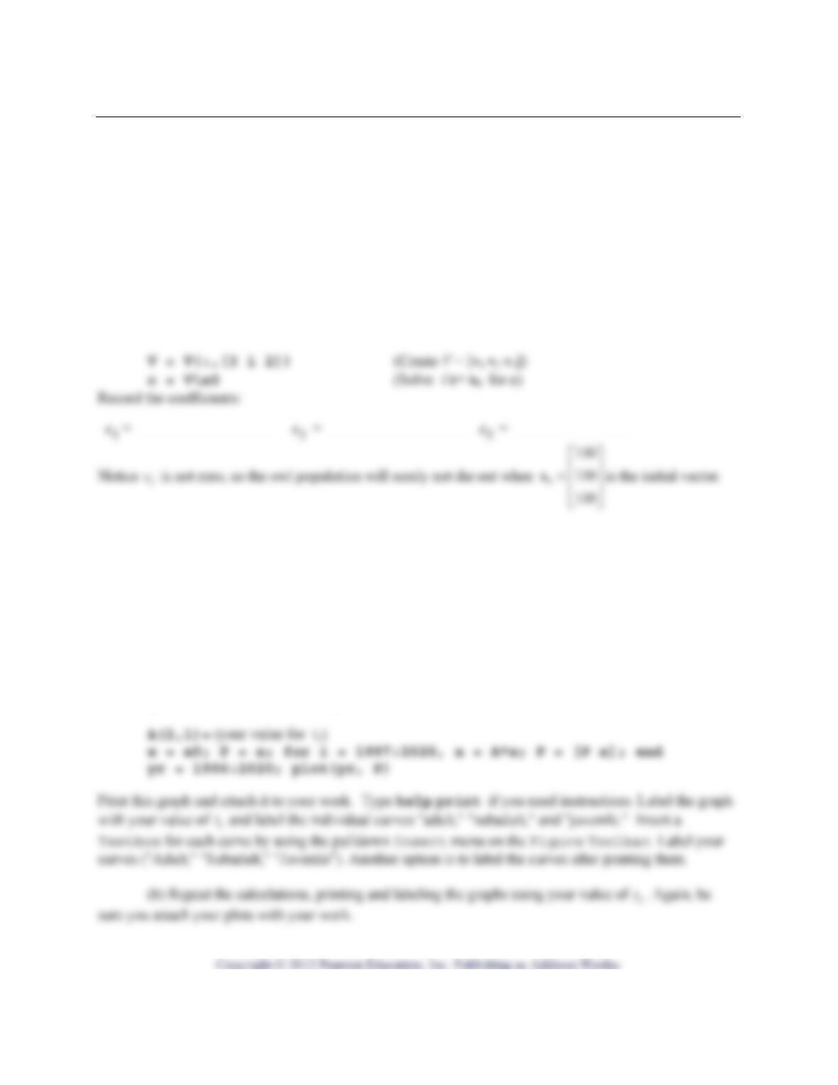
(a) Using t= 1
t, calculate and plot the values of k
j, k
s
, and k
afrom 1997 until 2020. The
following commands will do these things for t= 1
t:
Page 4 of 5 MATLAB Project: Using Eigenvalues to Study Spotted Owls
(c) Discuss what long term population trends your graphs show in the three age groups when t =
1
t, and what trends when t = 2
t. Are these the results you expected, based on what you know about the
dominant eigenvalue of the matrix A in each case?
4. (hand. Check to see if this problem is extra credit.) Let
00
00
0
a
At
bc
⎡
⎤
⎢
⎥
=
⎢
⎥
⎢
⎥
⎣
⎦
, and assume ,,,abctare positive.
(a) Let ( )f
λ
denote the characteristic polynomial of A. Calculate it and show work. You should
get 32
()
f
c abt
λλλ
=− + + .