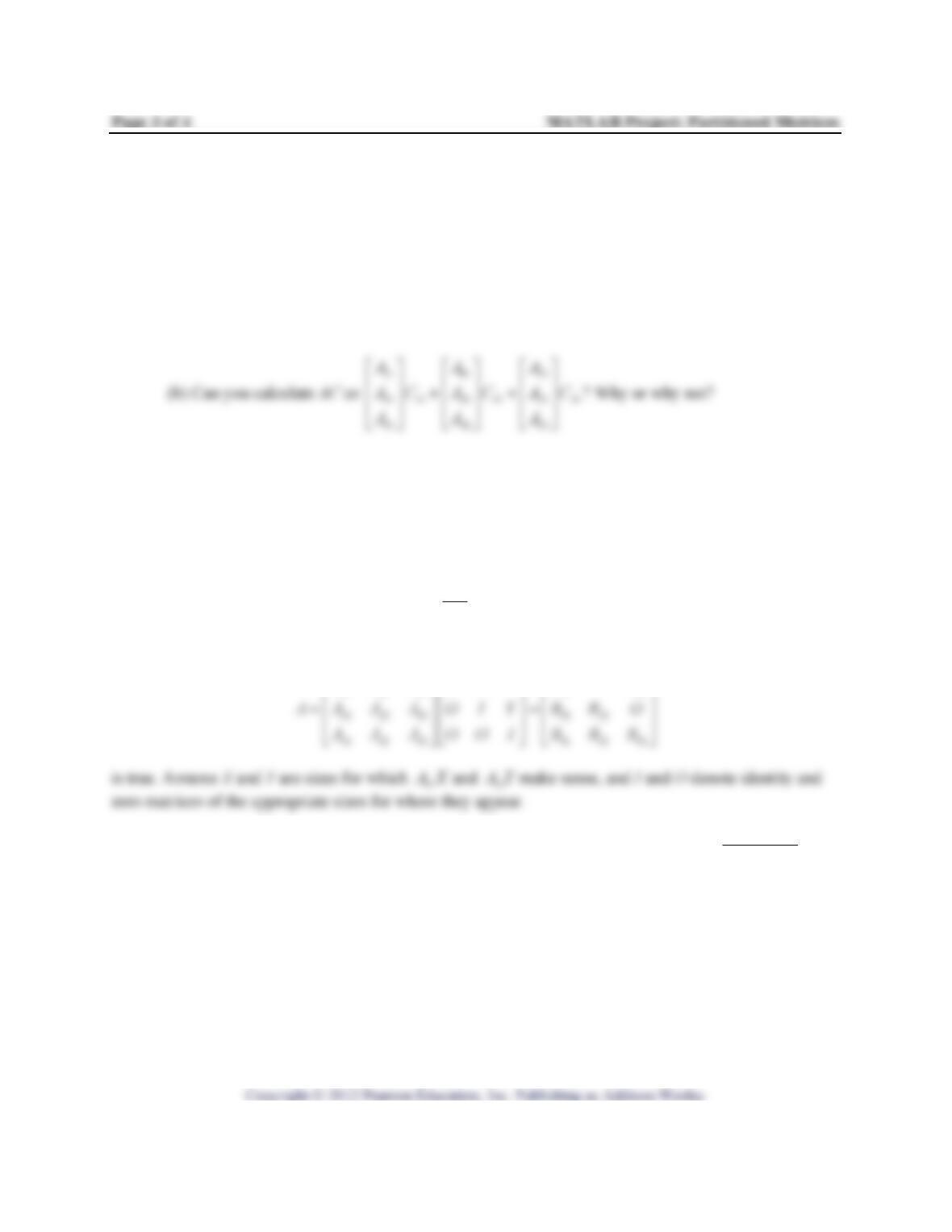
2. (hand) Using the matrices in question 1:
(a) Can you calculate AC as
11 11 21 12 31 13
11 21 21 22 31 23
11 31 21 32 31 33
CA CA CA
CA CA CA
CA CA CA
++
⎡⎤
⎢⎥
++
⎢⎥
⎢⎥
++
⎣⎦
? Why or why not?
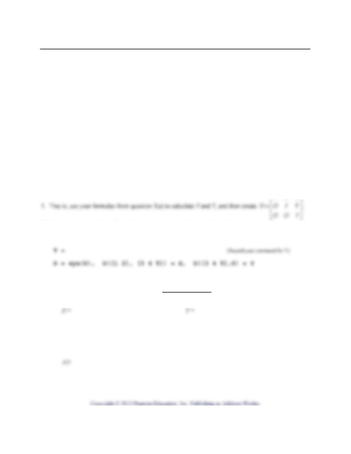
3. (hand) Now let
11 12 13
21 22 23
31 32 33
AAA
AAA A
AAA
⎡⎤
⎢⎥
=⎢⎥
⎢⎥
⎣⎦
denote any partitioned matrix in which 11
Aand 22
A are square
and invertible. We want formulas for X and Y so that
11 12 13 11 13
AAA IXO B OB
⎡⎤⎡⎤⎡⎤
(a) Find X and Y in terms of the ij
A
. Do the minimal amount of calculations and show work.
Page 4 of 4 MATLAB Project: Partitioned Matrices
(b) Find an additional condition on the blocks ij
A
so that 13
B
O=. Be careful. Do not write 1
12
A
−.
(Why not?) Show calculations:
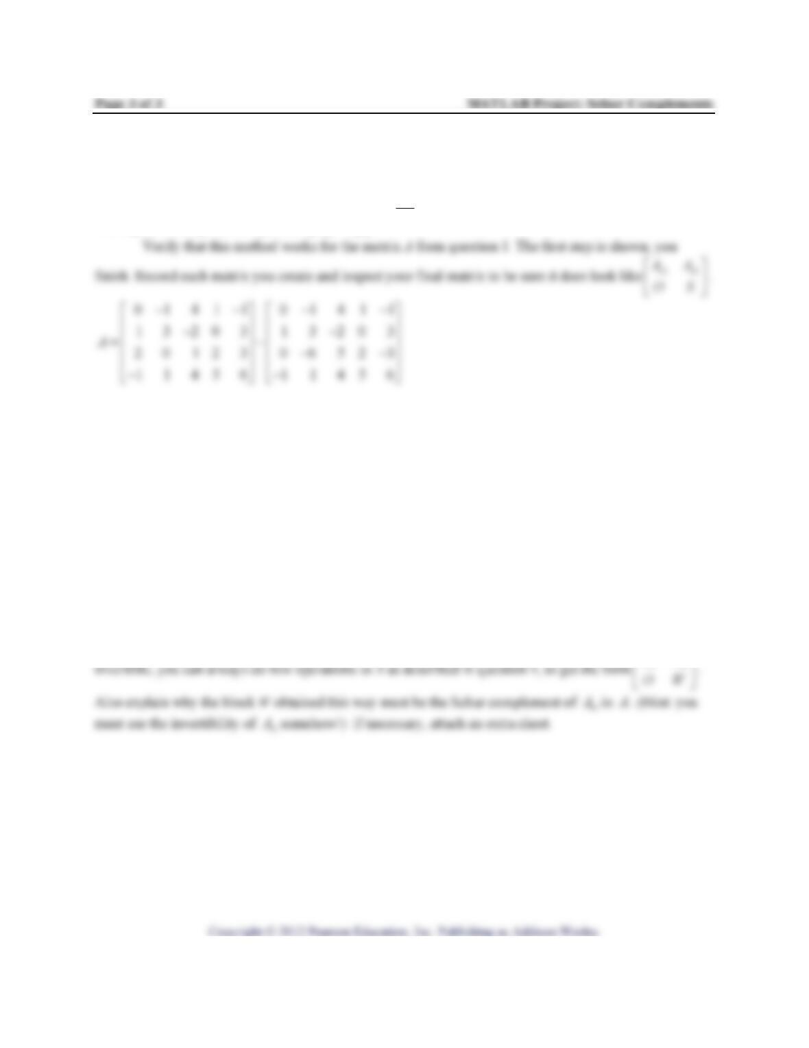
4. (MATLAB) Apply what you found in question 3 to the particular partitioned matrix A given in question
IXO
⎡⎤
We show a way to calculate X and D; you write a command to calculate Y:
X = -inv(A11)*A12
Record X and Y. Type A*D to calculate AD and mark the partitions in AD. Are the appropriate blocks
zero?
MATLAB Project: Schur Complements Name_______________________________
Purpose: To learn what Schur complements are and their connection with row reduction
Prerequisite: Section 2.4
MATLAB functions used: inv, eye, zeros, – , * ; and schurdat from Laydata4 Toolbox
Background. This is based on Exercise 16 in Section 2.4. Let 11 12
21 22
AA
AAA
⎡
⎤
=
⎢
⎥
⎣
⎦be a partitioned matrix in
⎡
⎢
⎣
1. (MATLAB) Type schurdat to get 11
01
13
A−
⎡
⎤
=
⎢
⎥
⎣
⎦, 12
41 1
20 3
A−
⎡
⎤
=
⎢
⎥
−
⎣
⎦, and 22
123
456
A⎡⎤
=⎢⎥
⎣⎦
. In
MATLAB they will be stored as A11, A12, A21, A22.
(b) One way to get the Schur complement S for the matrix here would be to just calculate it directly,
using the definition above. Type the following line to do that, and record the result:
Page 2 of 3 MATLAB Project: Schur Complements
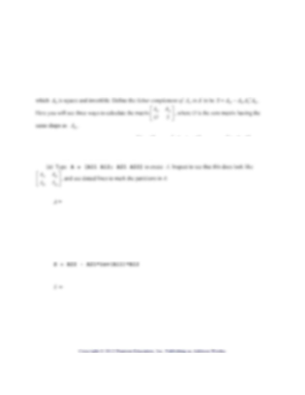
2. (hand) Assume now that 11 12
21 22
AA
AAA
⎡⎤
=⎢⎥
⎣⎦
is any partitioned matrix in which 11
Ais square and invertible.
⎡
⎢
⎣
3. (MATLAB) A second way to get the Schur complement S of 11
A
in
A
would be to use your formula
from question 2 to calculate L, then create IO
CLI
⎡
⎤
=
⎢
⎥
⎣
⎦, and then calculate CA. Do this for the matrix in
question 1. You figure out a command to calculate L and record your command below. A way is shown
to create C and CA:
L = (Record your command)
⎡
⎢
⎣
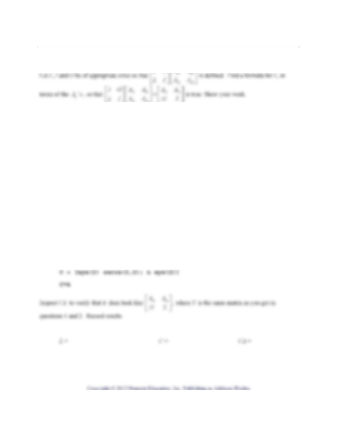
4. (hand) A third way to calculate the Schur complement S of 11
A
in A is to use row operations in a special
way. This method actually does the least arithmetic so is the most efficient method. Do not change
anything in
[
]
11 12
A
A but just add multiples of appropriate rows of
[
]
11 12
A
Ato rows of
[
]
21 22
A
Aso as
to create a block of zeros below 11
A
. Notice this is not the usual Row Reduction Algorithm because
nothing will change in the top block
[
]
11 12
A
A.
5. (hand) Assume now that 11 12
21 22
AA
AAA
⎡⎤
=⎢⎥
⎣⎦
is any partitioned matrix in which 11
A
is invertible. Prove that
the method described in question 4 will always work, to get a block of zeros below 11
A
. That is, if 11
A
is
A
A
AA
⎡⎤
MATLAB Project: LU Factorization Name_______________________________
Purpose: To practice Lay’s LU Factorization Algorithm and see how it is related to MATLAB’s
lu function.
Prerequisite: Section 2.5
MATLAB functions used: *, lu; and ludat and gauss from Laydata4 Toolbox
Background. In Section 2.5, read about Lay’s algorithm for calculating an LU factorization. Carefully
study Example 2. It is imperative you understand the algorithm for calculating the matrix L before
starting. In this project you will perform his algorithm on the matrices below, and see the connection
between his algorithm and the one used by MATLAB’s lu function.
534
⎢
⎢
⎢
⎢
⎢
⎣
−
⎡⎤
15 1 2
⎡⎤
13530
02311
−−
⎡
⎤
⎢
⎥
−−
2424
−−
⎡⎤
261
494
230
E
−
⎡⎤
⎢⎥
−−−
⎢⎥
=⎢⎥
−−
130
448
F
⎡⎤
⎢⎥
=⎢⎥
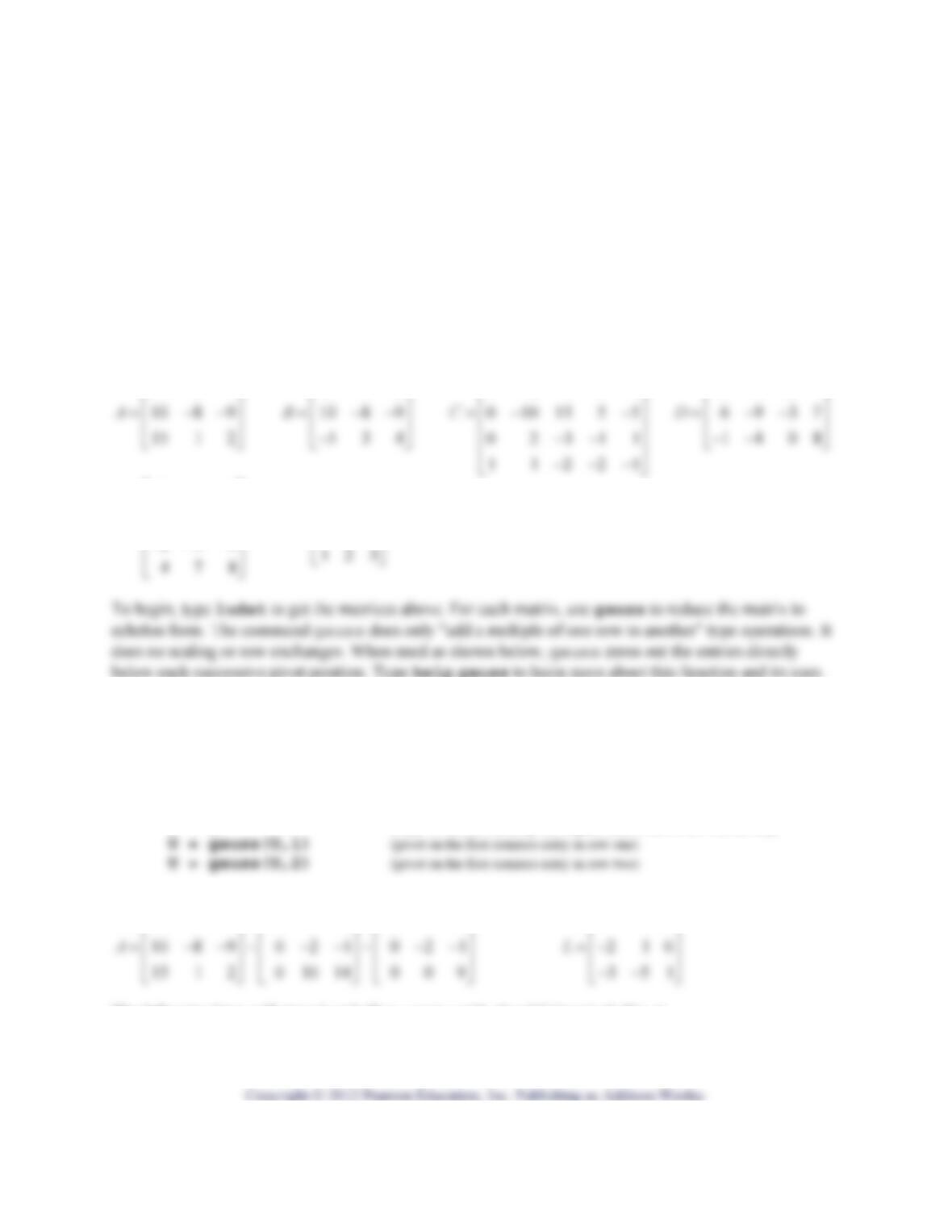
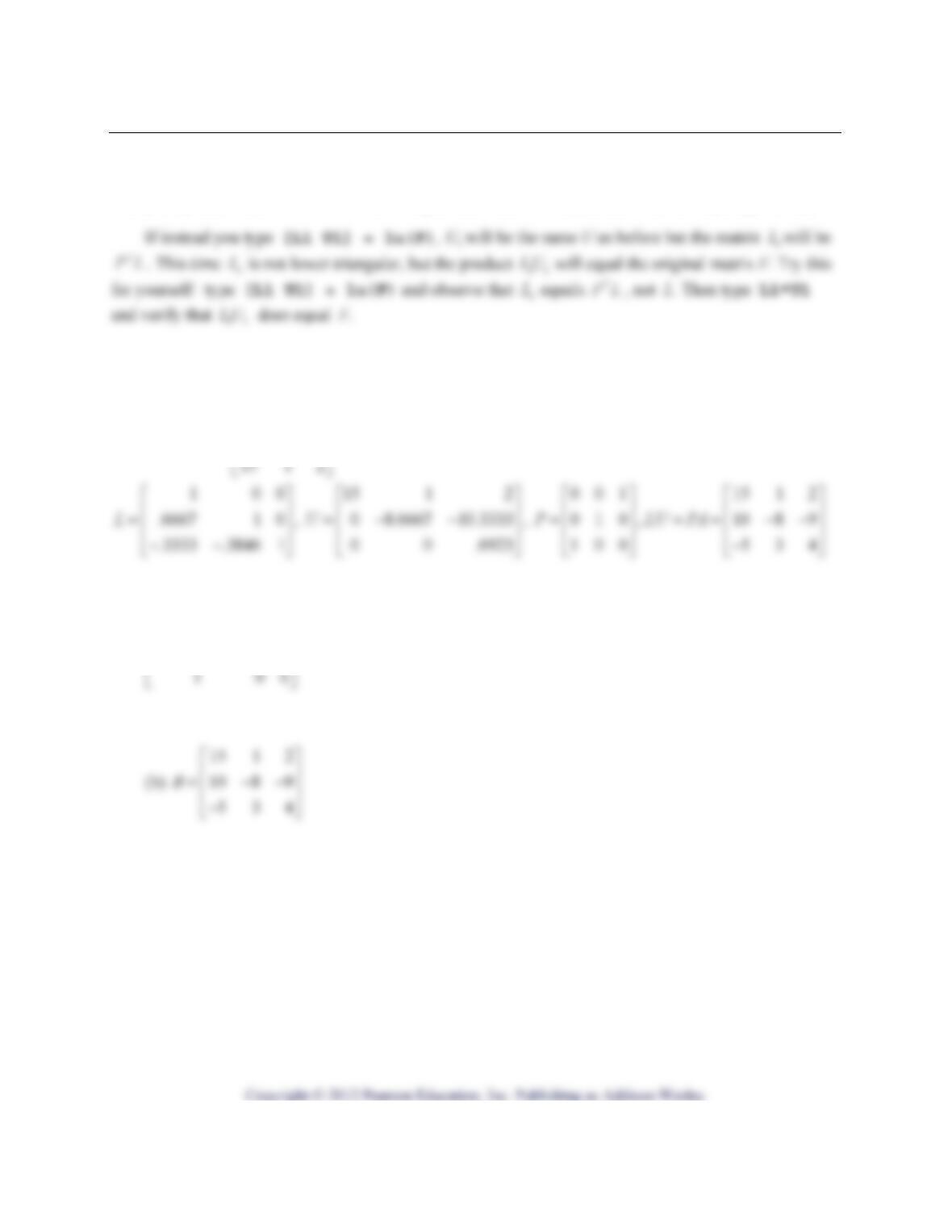
1. (MATLAB) For each matrix above, use gauss and the algorithm in Section 2.5 to calculate an LU
factorization. Record the matrix gotten from each gauss step. Inspect those to write L. Finally, verify
that LU does equal the original matrix (where U is the final matrix in your reduction).
(a) Here is the solution for A. We store each intermediate matrix as U, but the final U is what we really
want:
U = A (copy A so you can keep the original matrix and work with the copy
The matrices produced by the commands above: Inspecting the matrices on the left gives L:
534
⎢
⎢
⎢
⎣
−
⎡⎤
534
−
⎡⎤
534
−
⎡⎤
100
⎡
⎤
The following lines will store L and allow you to verify that LU does look like A:
L = [1 0 0;-2 1 0;-3 -5 1]
L*U, A

Page 2 of 6 MATLAB Project: LU Factorization
(b) Modify the commands above for the other matrices, and record the same type of information for each:
15 1 2
⎡⎤
(c) After two gauss steps on C you will see some zero rows. This simply means all multipliers are zero
after that, so put zeros in the positions that remain unfilled in L. Remember that L should have 1’s on
its diagonal.
13530
02311
−−
⎡⎤
⎢⎥
−−
1408
⎢⎥
−−
⎣⎦
261
−
⎡⎤
⎢⎥
2. (hand) Let A be the matrix from part 1 of this project and let
2
3
⎡
⎤
⎢
⎥
=
⎢
⎥
⎢
⎥
⎣
⎦
b. Solve Ax = b with the method
given in the beginning of section 2.5 of the text. The idea is that the following equations are equivalent:
Thus, if you first solve L=ybfor y and then U=xyfor x, you will have the solution to Ax = b. Do the
calculations by hand, and show work.
Step 1. Solve L=ybfor y by forward substitution:
Step 2. Using the vector y from Step 1, solve U=xyfor x by back substitution:
Background on MATLAB’s lu function. There are two ways to use lu, and we will illustrate these
with the matrix F above. Either way the result will not be an LU Factorization of the original matrix but
rather of a different matrix PF, where P is a permutation matrix. These matters are discussed a little more
in the Remarks at the bottom of page 6.
⎡
⎢
⎢
⎢
⎣
Page 5 of 6 MATLAB Project: LU Factorization
Try this for yourself: type [L U P]=lu(F) to see these matrices, and then type P*F,L*U to
verify for yourself that PF = LU is true. Compare the L and U obtained here with those you got in 1(f).
3. Use the lu function as just described with the matrices A, B, and C discussed earlier, and record
results. If necessary, recall these matrices by typing ludat. We do the first one as an example:
(a) For
534
10 8 9
A
−
⎡⎤
⎢⎥
=−−
⎢⎥
, first type [L U P] = lu(A), L*U, P*A and record the results:
Type [L1 U1] = lu(A), L1*U1,A and record the results:
1
.3333 .3846 1
.6667 1 0
L
−−
⎡⎤
⎢⎥
=⎢⎥
, 1
UU=,11
LU A=.
Page 6 of 6 MATLAB Project: LU Factorization
13530
02311
−−
⎡⎤
⎢⎥
−−
Remarks. A permutation matrix P is one obtained by rearranging the rows of an identity matrix. The
effect of calculating PA is to produce that same rearrangement of the rows of A .
MATLAB Project: An Economy with an Open Sector Name__________________________
Purpose: To study a linear system model of an open sector economy
Prerequisite: Section 2.6
MATLAB functions used: – , sum, eye; and ref from Laydata4 Toolbox
Background. This project is based on Exercise 13 in Section 2.6, where an economy with 7 production
sectors is described. Each sector produces goods and each uses some of the output of the other sectors.
()
1. Type the following lines to get the data for C and d and to calculate the column sums of C. Inspect the
output to be sure each entry of C and d is nonnegative and that each column sum of C is less than one:
c2s6
13
sum(C) (sum(C) yields a row vector containing the sum of each column)
Type the following lines to create IC−and to solve the equation
()
1
IC
−
−=xd
.
d = x =
Page 2 of 3 MATLAB Project: An Economy with an Open Sector
(b) Choose two more nonnegative demand vectors d1 and d2 and solve for the production vector
for each. Record all these vectors.
d1 = x1 = d2 = x2 =
2. Experiment to increase the (1,1) entry of C, until you find a new consumption matrix that gives a
solution with some negative entries – that is, until solving
()
IC−=xd
yields some negative entries in x.
Remember that to change the (1,1) entry of C to, say, .16, type C(1,1) = .16. Then use the arrow up
key to repeat the commands for M and R to find x.
MATLAB Project: Matrix Inverses and Infinite Series Name_______________________________
Purpose: To see examples for which the matrix series 23
ICC C++ + +… does converge to
1
()IC
−
− and examples for which it does not
Prerequisite: Section 2.6
MATLAB functions used: *, +, :, eye, for, end, format; and Laydata4 Toolbox
1. Use the matrix C which is defined in Exercise 13, Section 2.6. Type the following lines to get C and to
calculate 23 k
ICC C C++ + + +…for several values of k.
c2s6
13
Use the up arrow key ↑ to execute the sum line S=I+C*S repeatedly. Keep count as to how many times
the sum line is repeated and watch to see that this series does seem to converge. (The first time you
execute this line, you get SIC=+ ; the second time you get 2
SICC=+ + ; etc.) How many times must
you repeat it until the matrix S seems to stop changing, at least as far as what you see on the screen?
_________________
Definitions. The norm of a vector 12
(, , )
n
x
xx=x…is defined to be 22 2
12 n
x
xx=++x…. For example, if
x = [-4 2 –2 1], then ||x|| = 5. Clearly, the norm is a way to measure the size of a vector, and it is reasonable
to call a vector small if its norm is small. Notice that when a vector has only 2 or 3 entries, this is the same
definition of length you saw in analytic geometry.
2. If we had ( )ICSI−=, then S would be the multiplicative inverse for ( )IC−. Since we are dealing
with approximations, the question becomes, “Is S close enough to 1
()IC
−
−?” One way to check whether
Page 2 of 3 MATLAB Project: Matrix Inverses and Infinite Series
Experiment with different values of k to find how many terms of the series you must use in
2k
SICC C=+ + + +…in order to get the norm of ( )ICSI−−to be 10
10−or smaller.
Assuming that I is still in the workspace, the following lines calculate the norm of ( )ICSI−−for k = 10.
format short e
Do the same calculations for k = 20 and k = 30. Record the norm of ( )ICSI−−for each, in the following
table. Try larger values of k until you find one for which the norm of ( )ICSI−− is less than 10
10−, and
record that data as well.
k (number of
terms used)
10 20 30
Norm of
()ICSI−−
3. Find a 22×matrix C with nonnegative entries and some column sum greater than one, but for which it
still appears that the series 23
ICC C++ + +…converges to 1
()IC
−
−. Look for a simple 22×example!

Page 3 of 3 MATLAB Project: Matrix Inverses and Infinite Series
4. Find a matrix C with nonnegative entries for which 23
ICC C++ + +…definitely does not converge
to 1
()IC
−
− .
Again, look for a simple 22×example!
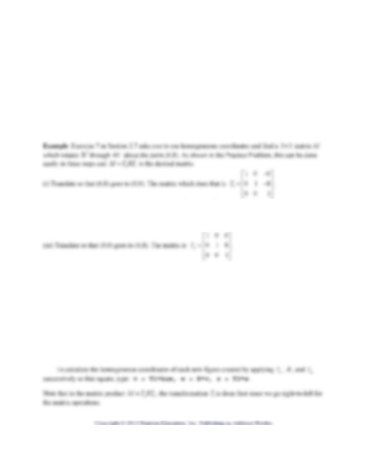
MATLAB Project: Homogeneous Coordinates for Computer Graphics Name_________________
Purpose: To practice using homogeneous coordinates to accomplish translations and other
transformations of 2
Prerequisite: Section 2.7
MATLAB functions used: + , * , cos, sin; and coordat and drawpoly from Laydata4 Toolbox
Background: The mathematics of computer graphics is closely tied to matrix multiplication.
Unfortunately, translating an object does not correspond directly to matrix multiplication because
translation is not a linear transformation. However, the use of homogeneous coordinates allows us to
accomplish translations and other transformations. Before you begin this project read about homogeneous
coordinates and study the Practice Problem in Section 2.7.
⎡
⎢
⎢
⎢
⎣
(ii) Rotate through 60about (0,0). The matrix is
0
0
001
cs
Rsc
−
⎡
⎤
⎢
⎥
=
⎢
⎥
⎢
⎥
⎣
⎦
where cos(60 )c=and sin(60 )s=.
1. (MATLAB) In this project you will use the M-file drawpoly, which draws polygons. To begin, type
coordat to get the matrices above and three others,
67766
88998
11111
box
⎡⎤
⎢⎥
=⎢⎥
⎢⎥
⎣⎦
,
2232
2332
1111
tri
⎡⎤
⎢⎥
=⎢⎥
⎢⎥
⎣⎦
, and
01100
200110
11111
box
⎡
⎤
⎢
⎥
=
⎢
⎥
⎢
⎥
⎣
⎦
.
The matrix box contains homogeneous coordinates for the vertices of the unit square whose lower
left vertex is at (6,8). A figure like this can be useful because sketching the effect of each successive
transformation on it can help you can see whether your matrices do accomplish the geometric effect you
want. Type drawpoly(box) to see this square.
Page 2 of 4 MATLAB Project: Homogeneous Coordinates for Computer Graphics
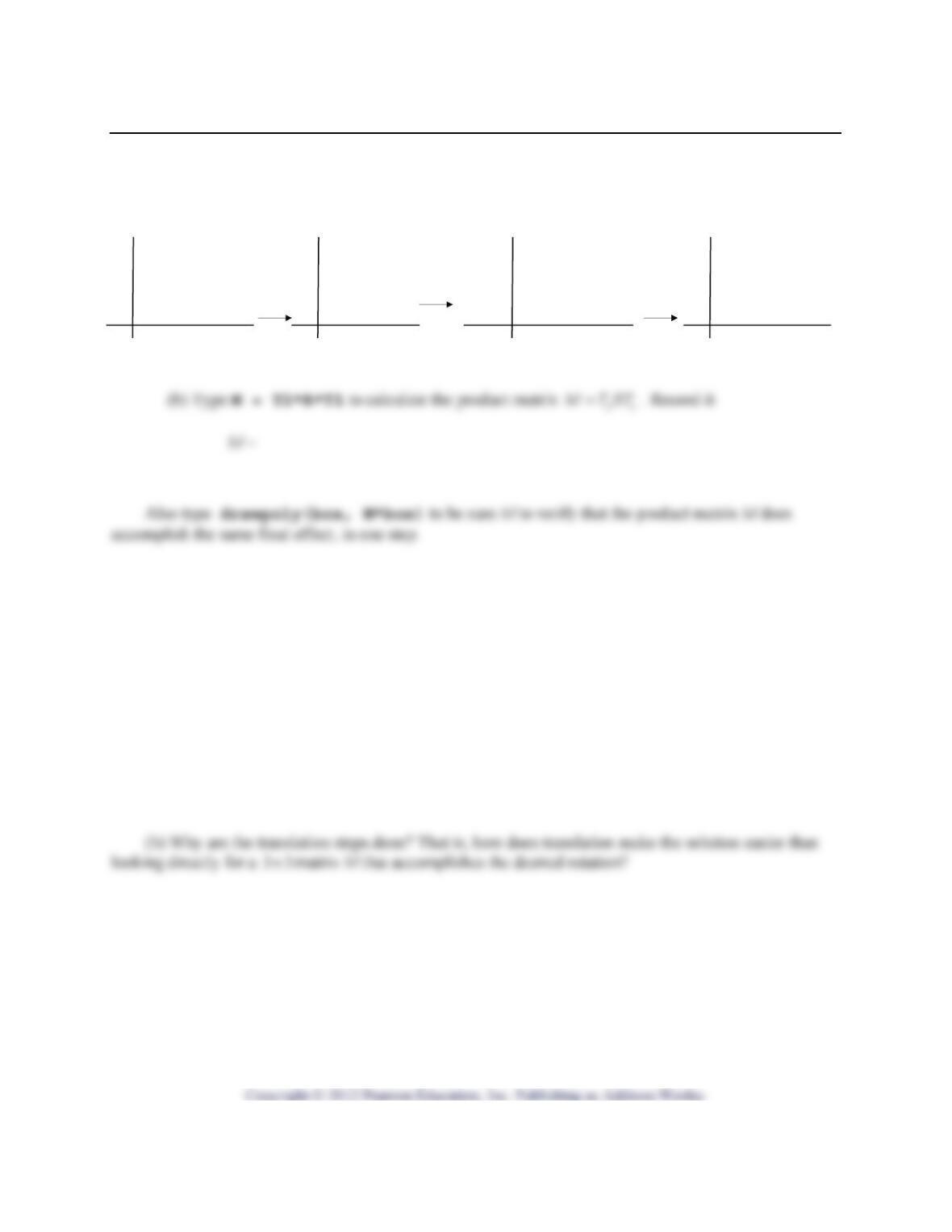
(a) Type drawpoly(box,v,w,z)to plot the original square and each transformation of it.
There will be a pause after each figure is graphed. Examine the figure, be sure you understand why it
looks like it does, and sketch the result below. Then press [Enter] to see the next figure.
2. (hand) Discuss example 1. Specifically:
(a) Why are homogeneous coordinates needed here? That is, why is it not possible to rotate 2
about a point like (6,8) using regular coordinates for points in 2
and a 22× matrix?
T1 RT2
Page 3 of 4 MATLAB Project: Homogeneous Coordinates for Computer Graphics
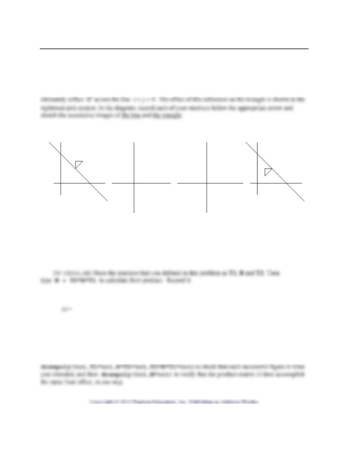
3. Consider the sketch below. On the leftmost axis system are sketched the line 4xy+=and the triangle
with vertices (2,2), (2,3) and (3,3). The coordinates of this triangle are stored in the matrix tri .
(a) (hand) Use ideas like those in question 1 above to find 33×matrices 1
T,
R
, and 2
Twhich
translate, reflect and translate so that applying them in succession to homogeneous coordinates will
1
T=
R
= 2
T=
Type drawpoly(tri) to check that tri contains homogeneous coordinates for the vertices of the
small triangle in the first sketch above. To verify that your matrices perform as desired, type