
3. The five matrices (A, B, C, D, and E ) can be loaded into a Maple session with the command:
cxeigdat( );. Recall that the Maple name for matrix D is DD. The eigenvectors command
can be used to obtain all eigenvalues and the corresponding eigenvectors for a matrix. Use the
following sequence of commands to construct the diagonal matrix L and invertible matrix P
with the property that AP = PL (the text calls the diagonal matrix D, but we already have a
matrix D in this project). Repeat these computations for the other four matrices. Report your
results in the table.
Matrix A B C D (i.e., DD) E
L
P
AP
PL
The results found in Questions 1–3 illustrate several important facts about eigenvectors and
eigenvalues. These are summarized here and are discussed in detail in Section 5.5 of the text.
Notes:
•Real-valued matrices can have complex-valued eigenvalues and eigenvectors.
Maple Project: Eigenvalue Analysis of the Spotted Owl NameMaple Project: Eigenvalue Analysis of the Spotted Owl NameMaple Project: Eigenvalue Analysis of the Spotted Owl Name
Purpose To complete the analysis of the spotted owl population, including
a determination of the critical juvenile survival rate that ensures
survival of the species.
Recall, from the Opening Example to Chapter 5 and Maple Project 6, “Initial Analysis of the
Spotted Owl”, that the spotted owl population is divided into three distinct life stages: first year
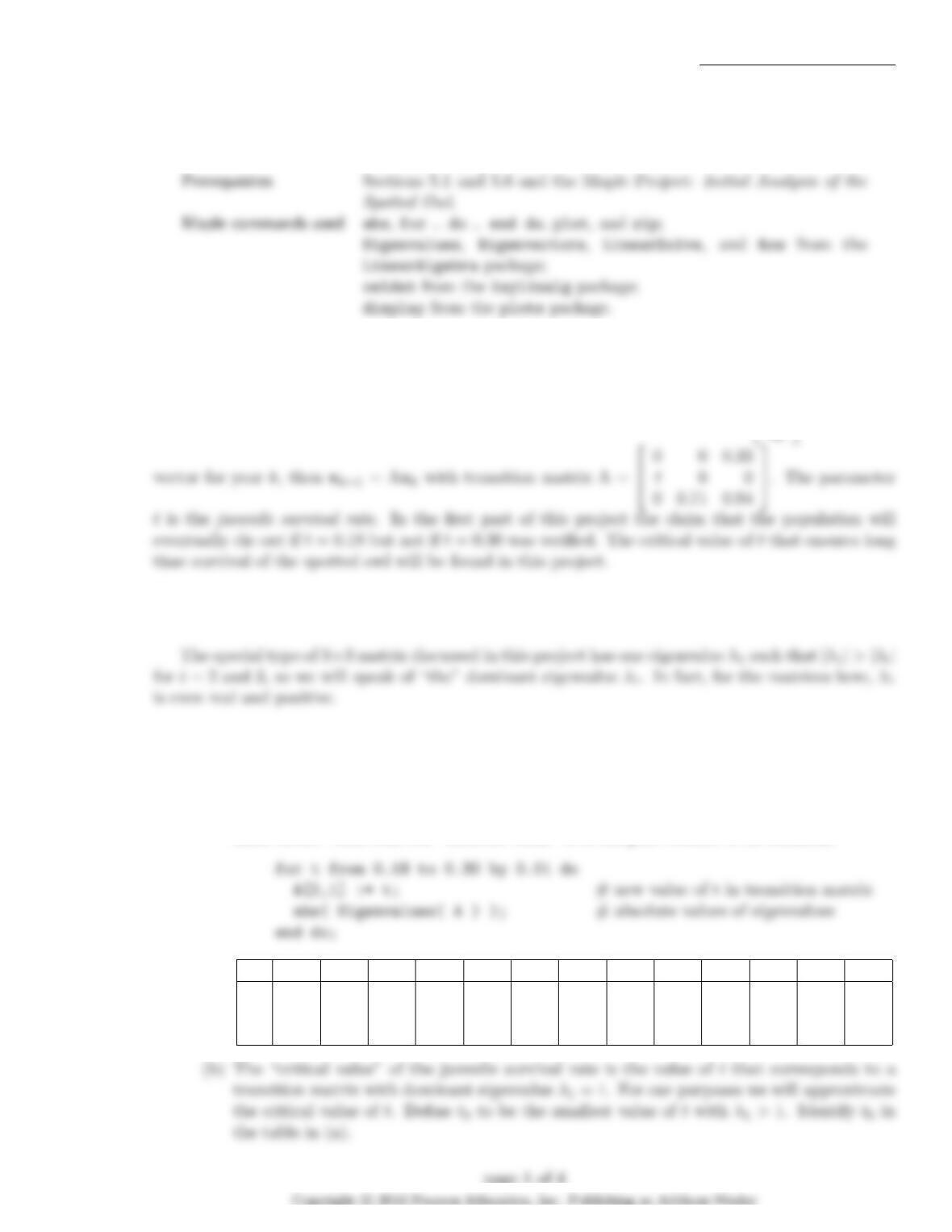
(juvenile), second year (subadult), and third year and beyond (adult). Let xk=
jk
sk
ak
be the state
Definition: Let A be an n×nmatrix with eigenvalues λ1,λ2, . . . , λnsorted so that |λ1| ≥ |λ2| ≥
. . . ≥ |λn|. The eigenvalue λ1is called a dominant eigenvalue of A.
1. Recall that the command: owldat( ); loads the transition matrix (and initial vector) for the
spotted owl into your current Maple session.
(a) Use the following Maple commands to find the dominant eigenvalue of the transition matrix
for t=0.18, 0.19, . . . , 0.30. Record these results, rounded to five significant digits, in the
table below. Note that the “absolute value” of a complex number is its modulus.
t0.18 0.19 0.20 0.21 0.22 0.23 0.24 0.25 0.26 0.27 0.28 0.29 0.30
λ1

2. Let A be the transition matrix with t=t0. Let v1,v2, and v3denote the eigenvectors of A, let
x0be an initial vector, and suppose c1,c2, and c3are scalars such that x0=c1v1+c2v2+c3v3.
(a) Explain why the population of owls will not die out if the coefficient of the eigenvector
corresponding to the dominant eigenvalue is not zero.
Hints:
•Do not find the eigenvectors or coefficients.
•The explanation depends on the properties of the dominant eigenvalue, etc., not their
specific values.
(b) Record the three eigenvalues, and their corresponding eigenvectors, v1,v2, and v3, of A in
the first row of the table at the bottom of this page. Notice that the dominant eigenvalue,
λ1, is real and positive and the other two eigenvalues, λ2and λ3, are complex conjugates.
c1c2c3
3. (a) Choose two new values of the juvenile survival rate t1and t2so that
t0−0.01 < t1< t0< t2< t0+ 0.01.
Report the eigenvalues and eigenvectors for the associated transition matrices in the second
and third rows of the following table. (Round all numbers to two significant digits.)
t λ1λ2λ3v1v2v3
t0=
t1=
t2=
Maple Project page 2 of 4 Eigenvalue Analysis of the Spotted Owl
Maple Project page 2 of 4 Eigenvalue Analysis of the Spotted Owl
Maple Project page 2 of 4 Eigenvalue Analysis of the Spotted Owl

(b) For each of these survival rates, t1and t2, create one graph showing the size of each
subpopulation for the years 1997 through 2020. Be sure each plot contains a caption that
indicates the value of t. Attach both plots to this project.
Hints:
•The first step is to generate the yearly populations for 1997 – 2020 when t= 0.30.
with(plots): # load plots package
A[2,1] := 0.30; # change juvenile survival rate
•The next set of Maple commands displays the size of each subpopulation for t= 0.30.
only minor modifications are needed for t1and t2.
yr := vector( [ $ 1997 .. 2020)] ):
ptJ := zip( (x, y) -> [x, y], yr, Row(P, 1) ): # juveniles
ptS := zip( (x, y) -> [x, y], yr, Row(P, 2) ): # subadults
ptA := zip( (x, y) -> [x, y], yr, Row(P, 3) ): # adults
(c) What trends in the three age groups are apparent in the graphs? How do the plots with
t=t1and t=t2differ? How are they similar? Are these results consistent with what you
know about the dominant eigenvalue of the transition matrix? (It might help to look at
the eigenvalues of the transition matrix for these values of t.)
Maple Project page 3 of 4 Eigenvalue Analysis of the Spotted Owl
Maple Project page 3 of 4 Eigenvalue Analysis of the Spotted Owl
Maple Project page 3 of 4 Eigenvalue Analysis of the Spotted Owl
Extra Credit
(a) Let A =
0 0 a
t0 0
0b c
, and assume a,b,c,tare positive. Show that f(λ) = −λ3+cλ2+abt
is the characteristic polynomial of A.
(b) Prove that A has one positive (real) eigenvalue and that the other two eigenvalues of A
must be complex conjugates. Let λ1denote the positive eigenvalue and let λ2and λ3
denote the other two eigenvalues.
Hints:
(c) Prove that λ1>|λ2|=|λ3|, hence the real positive eigenvalue of A will always be the
dominant eigenvalue for this type of matrix.
Hints:
•Show that f(λ) = (λ1−λ)(λ2−λ)(λ3−λ).
•Use this to show λ1λ2λ3=abt.
(d) Assume λ1= 1 and use this to obtain a formula for the exact critical value of t. Evaluate
your formula when a= 0.33, b= 0.71 and c= 0.94, and compare this with the critical
value you found experimentally in Question 1. Are they essentially the same? Discuss
what λ1= 1 means in the owl model. (For example, does it mean no births or deaths? If
not, then what?)

Maple Project: The Cayley-Hamilton Theorem NameMaple Project: The Cayley-Hamilton Theorem NameMaple Project: The Cayley-Hamilton Theorem Name
Purpose To learn about the Cayley-Hamilton Theorem
Prerequisites Section 5.2
Maple commands used eval;
Determinant and IdentityMatrix from the linalg package;
randomint from the laylinalg package.
Cayley–Hamilton Theorem: Every square matrix A satisfies its characteristic equation.
That is, if p(λ) = λn+cn−1λn−1+. . . +c1λ+c0is the characteristic polynomial for A, then
p(A) = 0. Note that 0 is the n×nzero matrix. To evaluate the characteristic polynomial “at a
matrix” it is essential to interpret the constant term, c0, as the corresponding multiple of the n×n
1. Empirical evidence of the validity of the Cayley–Hamilton Theorem can be obtained by looking
at randomly-selected matrices of various sizes. Use Maple to fill in the following table. (For
nAp(λ)p(A) – written as the sum of n+ 1 matrices
2
3
4
8
page 1 of 2
page 1 of 2
page 1 of 2

No content or questions on this page. Use this space for additional work if needed.
Maple Project page 2 of 2 The Cayley-Hamilton Theorem
Maple Project page 2 of 2 The Cayley-Hamilton Theorem
Maple Project page 2 of 2 The Cayley-Hamilton Theorem
Maple Project: Pseudo-Inverse of a Matrix NameMaple Project: Pseudo-Inverse of a Matrix NameMaple Project: Pseudo-Inverse of a Matrix Name
Purpose To investigate the pseudo-inverse of a matrix and its use in solving
overdetermined systems.
Notes:
•This definition of the pseudo-inverse applies only when (ATA) is invertible. This occurs if and
only if A has linearly independent columns. (Why?)
•The singular value decomposition can be used to define the pseudo-inverse of any matrix. (See
Example 7 in Section 7.4 of the text.)
1. Let A be an m×nmatrix and assume ATA is nonsingular. What size matrix is A+, the
pseudo-inverse of A?
2. Let A be a randomly-selected 4 ×4 matrix with integer entries. Use Maple to compute ATA
3. Repeat Question 2 with a randomly-selected 3 ×2 matrix with integer entries.
5. Repeat Question 2 with a randomly-selected 5 ×1 matrix with integer entries.
page 1 of 4
page 1 of 4
page 1 of 4

6. Examples 1 and 2 in Section 6.5 demonstrate that the “least-squares” solution to Ax=bis
(a) Show that, if A is invertible, then wis the exact solution, i.e., Aw=b.
(b) Show that, if bis in the range of A, then wis the exact solution.
Maple Project page 2 of 4 Pseudo-Inverse of a Matrix
Maple Project page 2 of 4 Pseudo-Inverse of a Matrix
Maple Project page 2 of 4 Pseudo-Inverse of a Matrix

(c) Consider the following system of linear equations:
5x1+ 6x2= 7
3x1−4x2= 8
2x1+ 9x2= 5
(d) Use the following template of Maple commands to graph the three lines. Then, identify
on a hardcopy of the graph, the point that corresponds to the vector w. You will need to
supply an appropriate viewing window to create the final graph. (Attach the final graph
to this project.)
with( plots ):
eq1 := 5*x1 + 6*x2 = 7;
Maple Project page 3 of 4 Pseudo-Inverse of a Matrix
Maple Project page 3 of 4 Pseudo-Inverse of a Matrix
Maple Project page 3 of 4 Pseudo-Inverse of a Matrix