
3. Let A = [v1v2. . . vk] be a matrix whose columns are v1,v2, . . . , vk. Explain why the
5. Examine the matrices B, C, D, and E in Question 1. For which of these matrices is the set of
its columns a linearly independent set?

6. Verify each of the following conclusions by hand or with Maple. Explain your method in the
space provided.
(a) Let v1=
2
3
5
1
,v2=
1
1
−2
9
,v3=
3
4
0
0
. Then {v1,v2,v3}is linearly independent
1
2
3
4
The matrix with these columns has rank 2.
(c) The set
1
4
6
1
,
2
5
9
11
,
4
6
12
1
,
4
6
15
1
is linearly independent because the rank of
1 4 6 1
2 5 9 11
4 6 12 1
4 6 15 1
is 4.
Maple Project page 4 of 4 Rank and Linear Independence
Maple Project page 4 of 4 Rank and Linear Independence
Maple Project page 4 of 4 Rank and Linear Independence

Maple Project: Population Migration NameMaple Project: Population Migration NameMaple Project: Population Migration Name
Purpose To study the population movement described in Exercise 11, Sec-
tion 1.10 in more detail.
Prerequisites Section 1.10
Notes:
•The Maple command to compute the matrix-vector product Ax is A.x.
•Large matrices can be viewed either with the matrix browser (click Browse in the context
menu) or after executing the command interface( rtablesize=infinity ): to force Maple
to display all matrices and vectors, regardless of their size.
1. To obtain the data for this exercise, load the laylinalg package into your current Maple
session with the command with( laylinalg ); then load the specific matrices for Exercise 11
in Section 1.9 with the command c1s10(11);.
(a) Record the values of Mand x0.
(b) Describe the calculations needed to produce the entries in M from the information in this
exercise.
page 1 of 4
page 1 of 4
page 1 of 4

2. Study the migration model described above. Use the following Maple commands to calculate
the population in California and in the rest of the US for the years 1990 – 2003 and store that
data as the columns of a matrix P.
x := x0/10.^6 : # rescale population data to millions
P := x: # put 1990 data in first column of P
Record the data from P in the table below. Round each number to 5 digits.
Population (in millions) assuming no external migration
Year 1990 1991 1992 1993 1994 1995 1996
California
Rest of US
Year 1997 1998 1999 2000 2001 2002 2003
California
Rest of US
Use the following Maple commands to plot the population in California, and the population in
the rest of the US, versus years, on the same graph. Include a printed copy of your graph with
this project.
with(plots): # load plots package
yr := < ($ 1990 .. 2003))] ); # vector [1990 1991 … 2003]
Maple Project page 2 of 4 Population Migration
Maple Project page 2 of 4 Population Migration
Maple Project page 2 of 4 Population Migration

3. Instead of assuming the total population is constant, suppose that the population in California
and the rest of the US is actually increasing each year because of immigration, say 0.1 million
Use the next set of Maple commands to calculate the new population predictions for 1990–2003.
d := < 0.1, 2.0 >: # annual immigration (in millions)
x := x0/10.^6 : # rescale population data to millions
P := x: # put 1990 data in first column of P
Record the data from P in the table below. Round each number to 5 digits.
Population (in millions) assuming external migration
Year 1990 1991 1992 1993 1994 1995 1996
California
Rest of US
Year 1997 1998 1999 2000 2001 2002 2003
California
Rest of US
Maple Project page 3 of 4 Population Migration
Maple Project page 3 of 4 Population Migration
Maple Project page 3 of 4 Population Migration

No content or questions on this page. Use this space for additional work if needed.
Maple Project page 4 of 4 Population Migration
Maple Project page 4 of 4 Population Migration
Maple Project page 4 of 4 Population Migration

Maple Project: Initial Analysis of the Spotted Owl NameMaple Project: Initial Analysis of the Spotted Owl NameMaple Project: Initial Analysis of the Spotted Owl Name
Purpose To study the owl population with several survival rates for juveniles.
Prerequisites Section 1.10 (and the Opening Example for Chapter 5)
The background information for this project can be found in the Opening Example to Chapter 5.
The fundamental idea is that spotted owls have three distinct life stages: first year (juvenile), second
year (subadult), and third year and beyond (adult) where jk,skand akdenote the number of owls
in each stage in year k. Let xk=
jk
sk
ak
and define the transition matrix A =
0 0 0.33
t0 0
0 0.71 0.94
.
1. Let t= 0.18 and suppose there are 100 owls in each life stage in 1997. Load the laylinalg
package, then use the command owldat(); to load the transition matrix, A, (with t= 0.18)
and the initial population vector, x0, in 1997.
(a) The population in each stage and the total population in 1998 can be found with the
following Maple commands:
x := x0; # initial population in 1997
Spotted owl population when the juvenile survival rate is t= 0.18
Year 1997 1998 1999 2000 2010 2020
Juvenile
Subadult
Adult
Total
page 1 of 4
page 1 of 4
page 1 of 4
(b) Continuing to execute these lines manually becomes tiresome (and it can be difficult to
keep track of the years as well). Instead, use the following repetition loop to calculate the
annual population vectors through 2020 and store the results in the matrix P.
x := x0; # initial population in 1997
A simple way to select the data needed to fill in the table is illustrated below:
T := SubMatrix( P, 1..-1, [1..4,14,24] ); # select cols of P
(c) The next set of Maple commands prepares and plots these results in a single graph. Include
this graph with your project.
with(plots): # load plots package
yr := Vector( [ $ 1997 .. 2020)] ):
ptJ := zip( (x, y) -> [x, y], yr, Row(P, 1) ): # points for juveniles
2. Repeat Question 1 with a juvenile survival rate of t= 0.30. To change the value of tin the
transition matrix A, use the command: A[2,1] := 0.30;.
Spotted owl population when the juvenile survival rate is t= 0.30

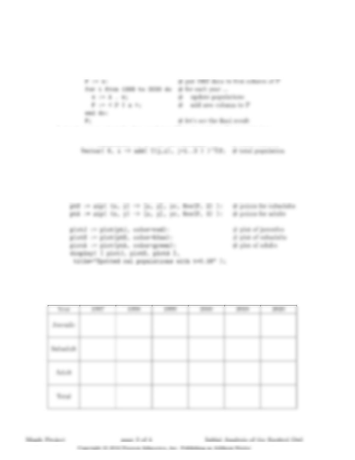
3. Create separate plots for the three spotted owl subpopulations when the juvenile survival rate
is t= 0.20, t= 0.24, t= 0.26, and t= 0.28.
Summarize how the three populations (and the total population) change between 1997 and
2020 for the different values of the juvenile survival rate. For what values of tdo you think the
owl will survive (forever)?


Maple Project: The Adjacency Matrix of a Graph NameMaple Project: The Adjacency Matrix of a Graph NameMaple Project: The Adjacency Matrix of a Graph Name
Example: Verify that matrix A is the adjacency matrix for the graph shown below.
12 6
3
5
010000
101001
010110
Theorem: (Interpretation of the powers of an adjacency matrix) If A is the adjacency matrix of
1. To understand why the theorem is true, we will examine – by hand – the (6,3) entry of A2. Using
the “Row-Column Rule”, the (6,3) entry of A2is a61a13+a62a23+a63a33+a64a43+a65a53+a66a63.

2. Observe that the product a62a23 = (1)(1) = 1 says that there is one length two path connecting
3. The adjacency matrix A for the graph shown above can be obtained with the commands:
(a) Find, and record, A2and A3.
A2A2
Maple Project page 2 of 4 The Adjacency Matrix of a Graph
Maple Project page 2 of 4 The Adjacency Matrix of a Graph
Maple Project page 2 of 4 The Adjacency Matrix of a Graph

(b) Notice that the (1,2) entry of A2is zero, so there are no paths of length two from node 1
to node 2. Verify this by studying the graph. Similarly, notice that the (6,6) entry of A3
i. How many paths of length two go from node 4 to itself? What are they?
ii. How many paths of length three go from node 4 to node 5? What are they?
iii. Which pair(s) of nodes are connected with the most paths of length 2? How many?
iv. Which pairs of nodes are not connected by any path of length 2 or 3? What are they?
(c) Suppose A is the adjacency matrix of a graph. Explain why you must calculate the sum
A + A2+. . . +Akin order to decide which pairs of nodes have contact level k?

4. Eight workers, denoted W1, .., W8, handle a potentially dangerous substance. Safety precau-
tions are taken, but accidents do happen occasionally. It is known that if a worker becomes
contaminated, s/he could spread this through contact with another worker. The graph below
shows which workers have direct contact with which other workers.
(a) Write the adjacency matrix A for the following graph:
W8 W7 W6
W5 W4
W
3
W2
W1
(b) Enter this adjacency matrix A in your Maple session and answer the following questions:
i. Which workers have contact level 3 with W3?
ii. Which workers have contact level 3 with W7?
(d) Define what is meant when a worker is “dangerous”. Be very specific so anyone could
decide whether a worker was “dangerous” according to your definition.
(e) Using your definition, answer the following questions. Be sure to explain your answers and
verify that they are consistent with your definition of “dangerous”.
i. Which workers are the most dangerous if contaminated?
ii. Which workers are the least dangerous if contaminated?

Maple Project: An Economy with an Open Sector NameMaple Project: An Economy with an Open Sector NameMaple Project: An Economy with an Open Sector Name
Notes:
•While Maple’s MatrixInverse command can be used to calculate the solution to any linear
system whose coefficient matrix is invertible, you are encouraged to use the MatrixInverse
command in this project.
1. Enter the consumption matrix, C, and final demand vector, d, in a Maple session. Assuming
the laylinalg package has been loaded, the command c2s6( 13 ); can be used to define C
and d.
(a) Verify that each column sum is less than one. The column sums of the 7 ×7 matrix C can
be found with the command:

2. Explain why it is important for the entries of the production vector to be nonnegative.
3. Use trial and error (and educated guessing) to find one entry in the first column of C which,
when changed to a different positive number, has the property that solving (I −C)x=dwith
modified C x
4. What do the numbers in your new matrix C say about the economy? Explain why your new
matrix produces a nonfeasible demand vector? (Be sure your explanation utilizes appropriate

Maple Project: Curve Fitting NameMaple Project: Curve Fitting NameMaple Project: Curve Fitting Name
Purpose To find the polynomial of order (n−1) that passes through ndata
points.
Prerequisites Section 2.2
Maple commands used convert,evalf,interp and plot;
Column,MatrixInverse, and VandermondeMatrix from the
LinearAlgebra package.
1. Find the n×nmatrix M.
2. Read about Vandermonde matrices in Exercise 11 in the Supplementary Exercises for Chapter 2
(see page ???). Under what conditions is the matrix M in Question 1 invertible?
3. Assuming M is nonsingular, the interpolation problem is solved by a= M−1y. Is the polynomial
through the points (x1, y1), (x2, y2), . . . , (xn, yn) unique? Why or why not?

4. Select a character string consisting of at least 8 letters. One possible source for the string is to
use your name – first, last, or a combination of the two.
Use the coding scheme given below to generate data points from your string.
a = -12 b = -11 c = -10 d = -9 e = -8 f = -7
g = -6 h = -5 i = -4 j = -3 k = -2 l = -1
m = 0 n = 1 o = 2 p = 3 q = 4 r = 5
s = 6 t = 7 u = 8 v = 9 w = 10 x = 11
y = 12 z = 13
(a) List the 8 data points.
i1 2 3 4 5 6 7 8
xi
yi
(b) Give the Maple commands you use to enter the vector yand the matrix M.
(c) What Maple command(s) did you use to find the coefficient vector a?
(d) What is the interpolating polynomial for your data?
Maple Project page 2 of 4 Curve Fitting
Maple Project page 2 of 4 Curve Fitting
Maple Project page 2 of 4 Curve Fitting

(e) Graph the interpolating polynomial for 1 ≤x≤8 on the axes provided. (Be sure to label
the axes.)
123456789
x
(f) Does the interpolating polynomial have any relative maxima or minima outside the interval
[1,8]? Explain.
–30 –25 –20 –15 –10 –5 5 10 15 20 25 30
x
Extra Credit Look at the online help for the interp command. Use this information to give a single Maple
command that returns the interpolating polynomial through the data points obtained from
your name. How does this compare with the interpolating polynomial you found?

No content or questions on this page. Use this space for additional work if needed.
Maple Project page 4 of 4 Curve Fitting
Maple Project page 4 of 4 Curve Fitting
Maple Project page 4 of 4 Curve Fitting