6.4 • Solutions 377
⎡
⎢
⎢
⎢
⎣
1/ 5 1/2 1/2
⎡⎤
⎢⎥
16. The columns of Q will be normalized versions of the vectors
1
v,
2
v, and
3
v found in Exercise 12.
Thus
⎢
⎢
⎢
⎣
1/2 1/(2 2) 1/2
287
1/2 1/(2 2) 1/2
⎡⎤
−
⎢⎥
⎡
⎤
−
⎢⎥
17. a. False. Scaling was used in Example 2, but the scale factor was nonzero.
18. a. False. The three orthogonal vectors must be nonzero to be a basis for a three-dimensional
subspace. (This was the case in Step 3 of the solution of Example 2.)
19. Suppose that x satisfies Rx = 0; then Q Rx = Q0 = 0, and Ax = 0. Since the columns of A are linearly
20. If y is in Col
A, then y = Ax for some x. Then y = QRx = Q(Rx), which shows that y is a linear
combination of the columns of Q using the entries in Rx as weights. Conversly, suppose that y = Qx
21. Denote the columns of Q by
1
{, , }
n
…
qq
. Note that n ≤ m, because A is m × n and has linearly
independent columns. The columns of Q can be extended to an orthonormal basis for
m
as follows.
Let
1
f be the first vector in the standard basis for
m
that is not in
1
Span{ , , },
nn
W=…
qq
let
378 CHAPTER 6 • Orthogonality and Least Squares
22. We may assume that
1
{, , }
p
…uu
is an orthonormal basis for W, by normalizing the vectors in the
23. Given A = QR, partition
[]
12
AAA=
, where
1
A
has p columns. Partition Q as
[]
12
QQQ=
where
1
Q
has p columns, and partition R as
11 12
22
,
RR
ROR
⎡
⎤
=
⎢
⎥
⎣
⎦
where
11
R
is a p × p matrix. Then
R
R
24. [M]
Call the columns of the matrix
1
x,
2
x,
3
x, and
4
x and perform the Gram-Schmidt process on
these vectors:
11
=
vx
⎢
⎢
⎢
⎢
⎢
⎢
⎣
3
⎡
⎤
⎢
⎢
⎢
⎢
⎢
⎣
6
0
⎡
⎤
⎢
⎥
43
41 42
44 1 2 34 1 2 3
11 2 2 33
11
(1)
22
⋅
⋅⋅ ⎛⎞
=− − − =− −− −−
⎜⎟
⋅⋅ ⋅ ⎝⎠
xv
xv xv
vx v v vx v v v
vv v v vv
0
5
0
0
⎡⎤
⎢⎥
⎢⎥
⎢⎥
=⎢⎥
⎢⎥
6.5 • Solutions 379
10 3 6 0
⎧⎫
−
⎡⎤⎡⎤⎡⎤⎡⎤
⎪⎪
⎢⎥⎢⎥⎢⎥⎢⎥
25. [M] The columns of Q will be normalized versions of the vectors
1
v,
2
v, and
3
v found in Exercise
24. Thus
⎢
⎢
⎢
⎢
⎢
⎣
1/2 1/2 1/ 3 0 20 20 10 10
⎡⎤
−
⎢⎥
−−
⎡
⎤
26. [M] In MATLAB, when A has n columns, suitable commands are
Q = A(:,1)/norm(A(:,1))
% The first column of Q
6.5 SOLUTIONS
Notes:
This is a core section – the basic geometric principles in this section provide the foundation
for all the applications in Sections 6.6–6.8. Yet this section need not take a full day. Each example
provides a stopping place. Theorem 13 and Example 1 are all that is needed for Section 6.6. Theorem 15,
however, gives an illustration of why the QR factorization is important. Example 4 is related to Exercise
17 in Section 6.6.
1. To find the normal equations and to find ˆ
x, compute
12
121 6 11
23
T
AA
−
⎡⎤
−− −
⎡⎤ ⎡⎤
⎢⎥
=−=
380 CHAPTER 6 • Orthogonality and Least Squares
a. The normal equations are
()
TT
AA A=xb
:
1
2
611 4
.
11 22 11
x
x
−−
⎡⎤
⎡
⎤⎡⎤
=
⎢⎥
⎢
⎥⎢⎥
−
⎣
⎦⎣⎦⎣⎦
b. Compute
1
1
6 11 4 22 11 4
1
ˆ
x( ) 11 22 11 11 6 11
TT
AA A
−
−
−− −
⎡ ⎤⎡⎤ ⎡ ⎤⎡⎤
== =
b
2. To find the normal equations and to find
ˆ,
x compute
21
222 128
20
103 810
23
T
AA
⎡⎤
−
⎡⎤ ⎡⎤
⎢⎥
=−=
⎢⎥ ⎢⎥
⎢⎥
⎣⎦ ⎣⎦
⎢⎥
⎣⎦
a. The normal equations are
()
TT
AA A=xb
:
1
2
12 8 24 .
810 2
x
x
−
⎡⎤
⎡
⎤⎡⎤
=
⎢⎥
⎢
⎥⎢⎥
−
⎣
⎦⎣⎦⎣⎦
b. Compute
3. To find the normal equations and to find ˆ
x, compute
3
11021 6
T
⎡⎤
⎢⎥
−
⎡⎤⎡⎤
⎢⎥
a. The normal equations are
()
TT
AA A=xb
:
1
2
66 6
642 6
x
x
⎡⎤
⎡
⎤⎡⎤
=
⎢⎥
⎢
⎥⎢⎥
−
⎣
⎦⎣⎦⎣⎦
6.5 • Solutions 381
66 6 4266
1
ˆ642 6 6 6 6
216
TT
−1
−1
−
⎡ ⎤⎡⎤ ⎡ ⎤⎡⎤
=(Α Α) Α = =
⎢ ⎥⎢⎥ ⎢ ⎥⎢⎥
−−−
⎣ ⎦⎣⎦ ⎣ ⎦⎣⎦
xb
4. To find the normal equations and to find ˆ
x, compute
13
111 33
11
311 311
11
T
AA
⎡⎤
⎡⎤ ⎡⎤
⎢⎥
=−=
⎢⎥ ⎢⎥
⎢⎥
−
⎣⎦ ⎣⎦
⎢⎥
⎣⎦
a. The normal equations are
()
TT
AA A=xb
:
1
2
33 6
311 14
x
x
⎡⎤
⎡
⎤⎡⎤
=
⎢⎥
⎢
⎥⎢⎥
⎣
⎦⎣⎦⎣⎦
b. Compute
6
ˆ11 14 14
TT
−1
−1
33 11−36
⎡ ⎤⎡⎤ ⎡ ⎤⎡⎤
1
=(Α Α) Α = =
⎢ ⎥⎢⎥ ⎢ ⎥⎢⎥
3−33
24
⎣ ⎦⎣⎦ ⎣ ⎦⎣⎦
xb
5. To find the least squares solutions to Ax = b, compute and row reduce the augmented matrix for the
system
TT
AA A=
xb:
42214 10 1 5
220 4 01 1 3
20210 00 0 0
TT
AA A
⎡
⎤⎡ ⎤
⎢
⎥⎢ ⎥
⎡⎤
=∼−−
⎣⎦
⎢
⎥⎢ ⎥
⎢
⎥⎢ ⎥
⎣
⎦⎣ ⎦
b
6. To find the least squares solutions to Ax = b, compute and row reduce the augmented matrix for the
system
TT
AA A=
xb:
63327 10 1 5
33012 01 1 1
30315 00 0 0
TT
AA A
⎡
⎤⎡ ⎤
⎢
⎥⎢ ⎥
⎡⎤
=∼−−
⎣⎦
⎢
⎥⎢ ⎥
⎢
⎥⎢ ⎥
⎣
⎦⎣ ⎦
b
382 CHAPTER 6 • Orthogonality and Least Squares
7. From Exercise 3,
12
12
,
03
⎢
⎣
⎢
⎣
A
−
⎡
⎤
⎢
⎥
−
⎢
⎥
=
⎢
⎥
⎢
⎥
3
1,
4
⎡
⎤
⎢
⎥
⎢
⎥
=
⎢
⎥
−
⎢
⎥
b
and
ˆ.
4/3
⎡
⎤
=
⎢
⎥
−1/3
⎣
⎦
x
Since
8. From Exercise 4,
13
11,
11
A
⎡
⎤
⎢
⎥
=−
⎢
⎥
⎢
⎥
⎣
⎦
5
1,
0
⎡⎤
⎢⎥
=⎢⎥
⎢⎥
⎣⎦
b
and
ˆ.
1
⎡
⎤
=
⎢
⎥
1
⎣
⎦
x
Since
9. (a) Because the columns
1
a and
2
a of A are orthogonal, the method of Example 4 may be used to
find
ˆ
b, the orthogonal projection of b onto Col A:
12
1212
11 2 2
151
21 2 1
ˆ311
77 7 7
240
⎡
⎤⎡⎤⎡⎤
⋅⋅
⎢
⎥⎢⎥⎢⎥
=+ =+=+=
⎢
⎥⎢⎥⎢⎥
⋅⋅
⎢
⎥⎢⎥⎢⎥
−
⎣
⎦⎣⎦⎣⎦
ba ba
ba aaa
aa a a
⎡
⎢
⎣
10. (a) Because the columns
1
a and
2
a of A are orthogonal, the method of Example 4 may be used to
find
ˆ
b, the orthogonal projection of b onto Col A:
⎢
⎢
⎢
⎣
124
⎡
⎤⎡⎤⎡⎤
(b) The vector ˆ
x contains the weights which must be placed on
1
a and
2
a to produce
ˆ
b. These
⎡
⎢
⎣
11. (a) Because the columns
1
a,
2
a and
3
a of A are orthogonal, the method of Example 4 may be used
to find
ˆ
b, the orthogonal projection of b onto Col A:
6.5 • Solutions 383
3
12
123123
11 2 2 3 3
21
ˆ0
33
⋅
⋅⋅
=+ + =++
⋅⋅ ⋅
ba
ba ba
ba a aaaa
aa a a aa
12. (a) Because the columns
1
a,
2
a and
3
a of A are orthogonal, the method of Example 4 may be used
to find
ˆ
b, the orthogonal projection of b onto Col A:
(b) The vector ˆ
x contains the weights which must be placed on
1
a,
2
a, and
3
a to produce
ˆ
b. These
13. One computes that
11 0
11 , 2 , || || 40
11 6
AAA
⎡⎤ ⎡⎤
⎢⎥ ⎢⎥
=− − = − =
⎢⎥ ⎢⎥
⎢⎥ ⎢⎥
−
⎣⎦ ⎣⎦
ububu
14. One computes that
32
⎡⎤ ⎡ ⎤
⎢⎥ ⎢ ⎥
384 CHAPTER 6 • Orthogonality and Least Squares
15. The least squares solution satisfies
ˆ.
T
RQ=xb
Since
35
01
R
⎡
⎤
=
⎢
⎥
⎣
⎦
and
7
1
T
Q
⎡⎤
=⎢⎥
−
⎣⎦
b
, the augmented
matrix for the system may be row reduced to find
16. The least squares solution satisfies
ˆ.
T
RQ=xb
Since
23
05
R
⎡
⎤
=
⎢
⎥
⎣
⎦
and
17 / 2
9/2
T
Q
⎡⎤
=⎢⎥
⎣⎦
b
, the augmented
matrix for the system may be row reduced to find
17. a. True. See the beginning of the section. The distance from Ax to b is || Ax – b ||.
b . True. See the comments about equation (1).
18. a. True. See the paragraph following the definition of a least-squares solution.
b . False. If ˆ
x is the least-squares solution, then Aˆ
x is the point in the column space of A closest to
b. See Figure 1 and the paragraph preceding it.
19. a. If Ax = 0, then
.
TT
AA A==
x00 This shows that Nul A is contained in
Nul .
T
AA
6.6 • Solutions 385
20. Suppose that Ax = 0. Then
.
TT
AA A==
x00 Since
T
AA is invertible, x must be 0. Hence the
21. a. If A has linearly independent columns, then the equation Ax = 0 has only the trivial solution. By
Exercise 19, the equation
T
AA =
x0 also has only the trivial solution. Since
T
AA is a square
matrix, it must be invertible by the Invertible Matrix Theorem.
22. Note that
T
AA has n columns because A does. Then by the Rank Theorem and Exercise 19,
23. By Theorem 14,
ˆˆ.
TT
AAAAA
−1
==( )bx b
The matrix
1
()
TT
AAA A
−
is sometimes called the hat–
24. Since in this case
,
T
AA I
=
the normal equations give
ˆ.
T
A=
xb
25. The normal equations are
22 6
,
22 6
x
y
⎡⎤⎡⎤⎡⎤
=
⎢⎥⎢⎥⎢⎥
whose solution is the set of all (x, y) such that x + y =
26. [M] Using .7 as an approximation for
2/2,
02
.353535aa=≈
and
1.5.a=
Using .707 as an
6.6 SOLUTIONS
Notes:
This section is a valuable reference for any person who works with data that requires statistical
analysis. Many graduate fields require such work. Science students in particular will benefit from
Example 1. The general linear model and the subsequent examples are aimed at students who may take a
multivariate statistics course. That may include more students than one might expect.
1. The design matrix X and the observation vector y are
10 1
11 1
,,
12 2
13 2
X
⎡⎤⎡⎤
⎢⎥⎢⎥
⎢⎥⎢⎥
==
⎢⎥⎢⎥
⎢⎥⎢⎥
⎢⎥⎢⎥
⎣⎦⎣⎦
y
2. The design matrix X and the observation vector y are
386 CHAPTER 6 • Orthogonality and Least Squares
11 0
⎡⎤⎡⎤
⎢⎥⎢⎥
3. The design matrix X and the observation vector y are
11 0
−
⎡⎤⎡⎤
⎢⎥⎢⎥
4. The design matrix X and the observation vector y are
12 3
13 2
,,
X
⎡⎤⎡⎤
⎢⎥⎢⎥
⎢⎥⎢⎥
==
y
5. If two data points have different x–coordinates, then the two columns of the design matrix X cannot
6. If the columns of X were linearly dependent, then the same dependence relation would hold for the
vectors in
3
formed from the top three entries in each column. That is, the columns of the matrix
6.6 • Solutions 387
7. a. The model that produces the correct least-squares fit is y = X
β
+
ε
where
⎢
⎢
⎢
1
4
⎢
11 1.8
24 2.7
416 3.8
⎡
⎤
⎡⎤⎡⎤
⎢
⎥
⎢⎥⎢⎥
⎢
⎥
⎢⎥⎢⎥
⎣
⎦
ε
ε
ε
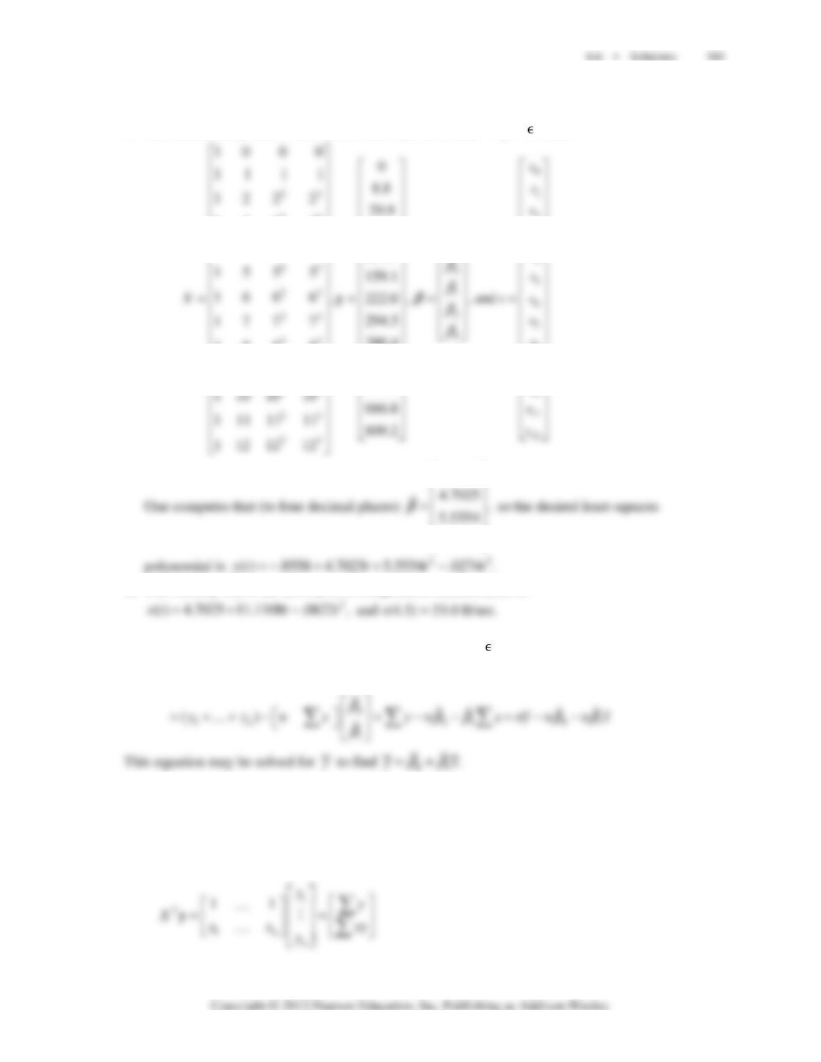
b. [M] One computes that (to two decimal places)
1.76
ˆ,
⎣
⎡
⎤
=
⎢
⎥
β
so the desired least-squares equation
8. a. The model that produces the correct least-squares fit is y = X
β
+ where
23
11 1 1 1 1
xx x y
β
⎡⎤
⎡⎤ ⎡⎤ ⎡⎤
ε
b . [M] For the given data,
416 64 1.58
6 36 216 2.08
8 64 512 2.5
⎡⎤⎡⎤
⎢⎥⎢⎥
⎢⎥⎢⎥
⎢⎥⎢⎥
so
1
.5132
ˆ( ) .03348 ,
TT
XX X
−
⎡⎤
⎢⎥
==−
y
β
and the least-squares curve is
9. The model that produces the correct least-squares fit is y = X
β
+ where
⎢
⎢
⎢
⎣
1
cos 1 sin 1 7.9
⎡
⎤
⎡⎤⎡⎤
ε
388 CHAPTER 6 • Orthogonality and Least Squares
10. a. The model that produces the correct least-squares fit is y = X
β
+ where
⎢
⎢
⎢
⎢
⎢
⎣
.02(10) .07(10)
1
.02(11) .07(11)
2
21.34
20.68
ee
ee M
−−
−−
⎡⎤
⎡
⎤
⎡⎤
⎢⎥
⎢
⎥
⎢⎥
⎢⎥
ε
ε
b. [M] One computes that (to two decimal places) 19.94
ˆ,
10.10
⎡
⎤
=
⎢
⎥
⎣
⎦
β
so the desired least-squares
11. [M] The model that produces the correct least-squares fit is y = X
β
+ where
⎢
⎢
⎢
⎢
⎢
⎣
1
2
13cos.88 3
1 2.3 cos1.1 2.3
⎡
⎤
⎡⎤⎡⎤
⎢
⎥
⎢⎥⎢⎥
ε
ε
One computes that (to two decimal places) 1.45
ˆ
.811
⎡
⎤
=
⎢
⎥
⎣
⎦
β
. Since e = .811 < 1 the orbit is an ellipse. The
12. [M] The model that produces the correct least-squares fit is y = X
β
+ ,ε where
⎢
⎢
⎢
1
4
5
13.78 91
14.11 98
14.73 110
14.88 112
⎡
⎤
⎡⎤⎡⎤
⎢
⎥
⎢⎥⎢⎥
⎢
⎥
⎢⎥⎢⎥
⎢
⎥
⎢⎥⎢⎥
⎣⎦⎣⎦
⎣
⎦
ε
ε
ε
ε
⎡
⎢
⎣
13. [M]
a. The model that produces the correct least-squares fit is y = X
β
+ where
⎢
⎢
⎢
⎢
⎢
⎢
⎡
⎢
⎢
⎢
23
23
23
23
⎢
⎢
⎢
⎢
⎣
133 3 62.0
144 4 104.7
380.4
188 8
471.1
199 9
571.7
⎢⎥
⎢
⎢⎥
⎢
⎢⎥
⎢
⎢⎥
⎢⎥
⎢⎥
2
3
8
9
10
⎢
⎥
⎥
⎢
⎥
⎥
⎢
⎥
⎥
⎢
⎥
⎢⎥
⎢
⎥
⎢⎥
⎢
⎥
⎢⎥
ε
ε
ε
ε
ε
⎢
⎢
⎢
.8558
.0274
−
⎡
⎤
⎢
⎥
−
⎢
⎥
⎣
⎦
b. The velocity v(t) is the derivative of the position function y(t), so
14. Write the design matrix as
[]
.1x
Since the residual vector = y – X
ˆ
β
is orthogonal to Col X,
ˆˆ
0()()
TT
XX=⋅=⋅ − = −11y 1y1ε
ββ
15. From equation (1) on page 369,
1
2
1
1
11
1
T
n
n
xnx
XX xx xx
x
⎡⎤
⎡
⎤
…
⎡⎤
⎢⎥
==
⎢
⎥
⎢⎥
⎢⎥
…
⎢
⎥
⎣⎦
⎣
⎦
⎢⎥
⎣⎦
∑
∑
∑
##
390 CHAPTER 6 • Orthogonality and Least Squares
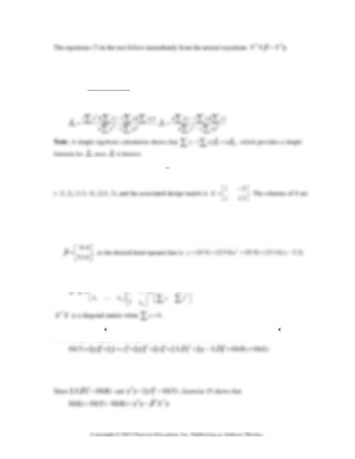
16. The determinant of the coefficient matrix of the equations in (7) is
22
().nx x−
∑
∑
Using the 2 × 2
formula for the inverse of the coefficient matrix,
2
0
22
1
ˆ1
ˆ()
y
xx
xy
xn
nx x
β
β
⎡⎤ ⎡⎤
⎡
⎤
−
=
⎢⎥ ⎢⎥
⎢
⎥
−
−⎢⎥
⎢⎥
⎣
⎦
⎣⎦
⎣⎦
∑
∑∑
∑
∑
∑∑
Hence
∑
β
β
0
1
17. a. The mean of the data in Example 1 is 5.5,x= so the data in mean-deviation form are (–3.5, 1),
⎢
⎢
⎢
13.5
12.5
−
⎡
⎤
⎢
⎥
⎢
⎥
⎣
⎦
orthogonal because the entries in the second column sum to 0.
b. The normal equations are
,
TT
XX X=y
β
or
0
1
40 9
.
021 7.5
β
β
⎡⎤
⎡
⎤⎡⎤
=
⎢⎥
⎢
⎥⎢⎥
⎣
⎦⎣⎦⎣⎦ One computes that
18. Since
⎢
⎢
⎣
∑
1
1
11
T
xnx
⎡⎤
⎡
⎤
…
⎡⎤
⎢⎥
∑
19. The residual vector = y –
ˆ
X
β
is orthogonal to Col X, while
ˆ
y
=X
ˆ
β
is in Col X. Since and
ˆ
y
are
thus orthogonal, apply the Pythagorean Theorem to these vectors to obtain
20. Since
ˆ
β
satisfies the normal equations,
ˆ,
TT
XX X=y
β
and
2
ˆˆˆˆˆˆ
|| || ( ) ( )
TTTTT
XXX XXX===y
ββββββ