6.7 • Solutions 391
6.7 SOLUTIONS
Notes
: The three types of inner products described here (in Examples 1, 2, and 7) are matched by
examples in Section 6.8. It is possible to spend just one day on selected portions of both sections.
Example 1 matches the weighted least squares in Section 6.8. Examples 2–6 are applied to trend analysis
in Seciton 6.8. This material is aimed at students who have not had much calculus or who intend to take
more than one course in statistics.
For students who have seen some calculus, Example 7 is needed to develop the Fourier series in
Section 6.8. Example 8 is used to motivate the inner product on C[a, b]. The Cauchy-Schwarz and
triangle inequalities are not used here, but they should be part of the training of every mathematics
student.
1. The inner product is
11 2 2
,4 5xy xy xy〈〉=+
. Let x = (1, 1), y = (5, –1).
a. Since
2
|| || , 9,xx=〈〉=x
|| x || = 3. Since
2
|| || , 105,yy=〈〉=y
|| || 105.=y
Finally,
22
|, |15 225.xy〈〉==
2. The inner product is
11 2 2
,4 5.xy xy xy〈〉=+
Let x = (3, –2), y = (–2, 1). Compute that
3. The inner product is 〈 p, q〉 = p(–1)q(–1) + p(0)q(0) + p(1)q(1), so
4. The inner product is 〈 p, q〉 = p(–1)q(–1) + p(0)q(0) + p(1)q(1), so
22
3,32tt t
〈
−+〉=
5. The inner product is 〈 p, q〉 = p(–1)q(–1) + p(0)q(0) + p(1)q(1), so
222
, 4,4 34550pp t t〈〉=〈++〉=++=
and
|| || , 50 5 2ppp=〈〉==
. Likewise
6. The inner product is 〈 p, q〉 = p(–1)q(–1) + p(0)q(0) + p(1)q(1), so
22
,3,3pp tt tt
〈
〉=〈−−〉=
〈
7. The orthogonal projection
ˆ
q
of q onto the subspace spanned by p is
8. The orthogonal projection
ˆ
q
of q onto the subspace spanned by p is
392 CHAPTER 6 • Orthogonality and Least Squares
9. The inner product is 〈p, q〉 = p(–3)q(–3) + p(–1)q(–1) + p(1)q(1) + p(3)q(3).
a. The orthogonal projection
ˆ
p
2
of
2
p
onto the subspace spanned by
0
p
and
1
p
is
b. The vector
2
ˆ
qp p t
2
2
=−=−5
will be orthogonal to both
0
p
and
1
p
and
01
{,,}ppq
will be an
10. The best approximation to
3
pt=
by vectors in
01
Span{ , , }Wppq=
will be
11. The orthogonal projection of
3
pt=
onto
012
Span{ , , }Wppp=
will be
12. Let
012
Span{ , , }.Wppp=
The vector
3
3
proj (17 / 5)
W
pp pt t=− =−
will make
0123
{,, ,}pppp
an orthogonal basis for the subspace
3
of
4
. The vector of values for
3
p
at (–2, –1, 0, 1, 2) is
13. Suppose that A is invertible and that 〈u, v〉 = (Au) ⋅ (Av) for u and v in
n
. Check each axiom in the
definition on page 376, using the properties of the dot product.
i. 〈u, v〉 = (Au) ⋅ (Av) = (Av) ⋅ (Au) = 〈v, u〉
14. Suppose that T is a one-to-one linear transformation from a vector space V into
n
and that 〈u, v〉 =
T(u) ⋅ T(v) for u and v in
n
. Check each axiom in the definition on page 376, using the properties of
the dot product and T. The linearity of T is used often in the following.
i. 〈u, v〉 = T(u) ⋅ T(v) = T(v) ⋅ T(u) = 〈v, u〉

15. Using Axioms 1 and 3, 〈u, c
v〉 = 〈c
v, u〉 = c〈v, u〉 = c〈u, v〉.
16. Using Axioms 1, 2 and 3,
2
|| || , , ,−=〈−−〉=〈−〉−〈−〉uv uvuv uuv vuv
17. Following the method in Exercise 16,
2
|| || , , ,+=〈++〉=〈+〉+〈+〉uv uvuv uuv vuv
18. In Exercises 16 and 17, it has been shown that
22 2
|| || || || 2 , || ||−= −〈〉+uv u uv v
and
2
|| ||+=uv
19. let
a
b
⎡⎤
=⎢⎥
⎢⎥
⎣⎦
u
and
.
b
a
⎡
⎤
=
⎢
⎥
⎢
⎥
⎣
⎦
v
Then
2
|| || ,ab=+u
2
|| || ,ab=+v
and
,2.ab〈〉=uv
Since a and b are
nonnegative,
|| || ,ab=+u
|| || .ab=+v
Plugging these values into the Cauchy-Schwarz
inequality gives
20. The Cauchy-Schwarz inequality may be altered by dividing both sides of the inequality by 2 and then
squaring both sides of the inequality. The result is
222
,||||||||
24
〈〉
⎛⎞
≤
⎜⎟
⎝⎠
uv u v
21. The inner product is
1
0
,()().fg ftgtdt〈〉=
∫
Let
2
() 1 3 ,ft t=−
3
() .gt t t=−
Then
22. The inner product is
1
0
,()().fg ftgtdt〈〉=
∫
Let f (t) = 5t – 3,
32
() .gt t t=−
Then
394 CHAPTER 6 • Orthogonality and Least Squares
23. The inner product is
1
0
,()(),fg ftgtdt〈〉=
∫
so
11
22 4 2
00
,(13) 9614/5,ff t dt t t dt〈〉=− = −+=
∫∫
and
|| || , 2 / 5.fff=〈〉=
24. The inner product is
1
0
,()(),fg ftgtdt〈〉=
∫
so
11
322 6 54
00
, ( ) 2 1/105,gg t t dt t t tdt〈〉=− =−+=
∫∫
and
|| || , 1/ 105.ggg=〈〉=
25. The inner product is
1
1
,()().fg ftgtdt
−
〈〉=
∫
Then 1 and t are orthogonal because
1
1
1, 0.ttdt
−
〈〉==
∫
So 1 and t can be in an orthogonal basis for
2
Span{1, , }.tt
By the Gram-Schmidt process, the third
basis element in the orthogonal basis can be
26. The inner product is
2
2
,()().fg ftgtdt
−
〈〉=
∫
Then 1 and t are orthogonal because
2
2
1, 0.ttdt
−
〈〉==
∫
So 1 and t can be in an orthogonal basis for
2
Span{1, , }.tt
By the Gram-Schmidt process, the third
basis element in the orthogonal basis can be
27. [M] The new orthogonal polynomials are multiples of
3
17 5tt−+
and
24
72 155 35 .tt−+
These
polynomials may be scaled so that their values at –2, –1, 0, 1, and 2 are small integers.
28. [M] The orthogonal basis is
0
() 1,ft=
1
() cos ,ft t=
2
2
( ) cos (1/ 2) (1/ 2)cos 2 ,ft t t=−=
and
6.8 SOLUTIONS
Notes
: The connections between this section and Section 6.7 are described in the notes for that section.
For my junior-senior class, I spend three days on the following topics: Theorems 13 and 15 in Section 6.5,
plus Examples 1, 3, and 5; Example 1 in Section 6.6; Examples 2 and 3 in Section 6.7, with the
motivation for the definite integral; and Fourier series in Section 6.8.
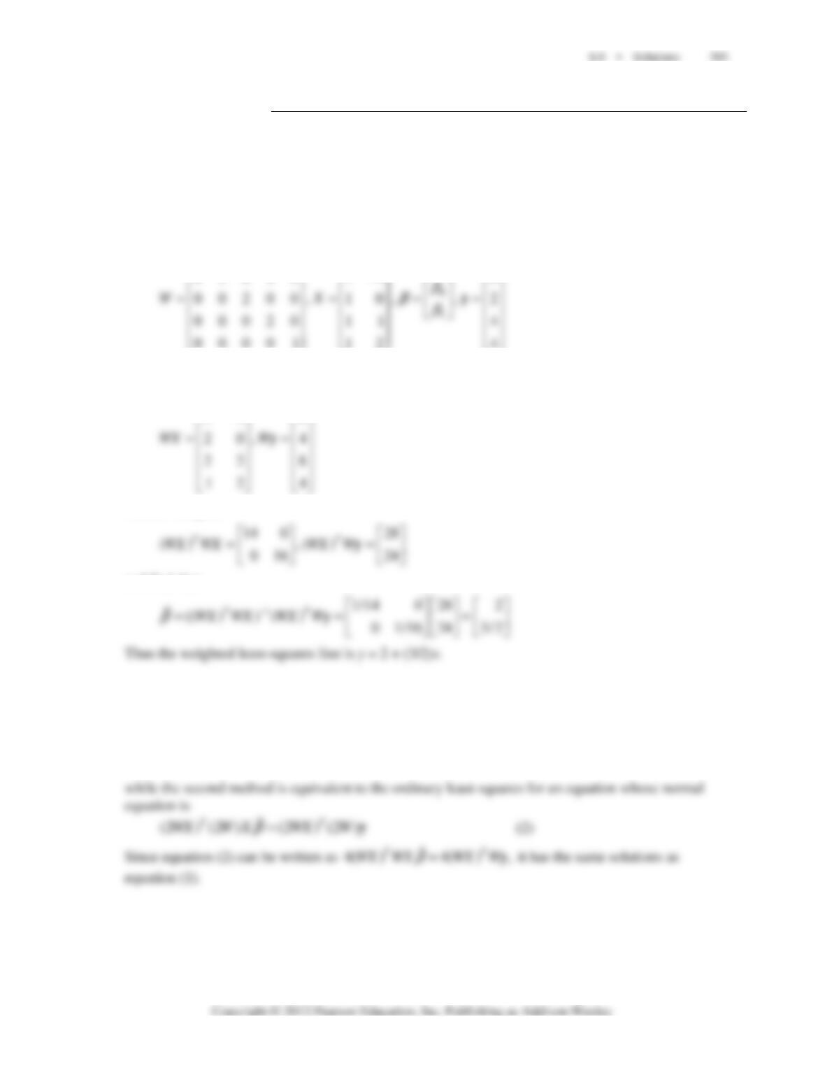
1. The weighting matrix W, design matrix X, parameter vector
β
, and observation vector y are:
10000 1 2 0
02000 1 1 0
−
⎡⎤⎡⎤⎡⎤
⎢⎥⎢⎥⎢⎥
−
⎣⎦⎣⎦⎣⎦
The design matrix X and the observation vector y are scaled by W:
12 0
22 0
−
⎡⎤⎡⎤
⎢⎥⎢⎥
−
Further compute
and find that
2. Let X be the original design matrix, and let y be the original observation vector. Let W be the
weighting matrix for the first method. Then 2W is the weighting matrix for the second method. The
weighted least-squares by the first method is equivalent to the ordinary least-squares for an equation
whose normal equation is
ˆ
() ()
TT
WX WX WX W=y
β
(1)
396 CHAPTER 6 • Orthogonality and Least Squares
3. From Example 2 and the statement of the problem,
0
() 1,pt=
1
() ,pt t=
2
2
() 2,pt t=−
3
3
() (5/6) (17/6),pt t t=−
and g = (3, 5, 5, 4, 3). The cubic trend function for g is the orthogonal
projection
ˆ
p
of g onto the subspace spanned by
0
,p
1
,p
2
,p
and
3
:p
03
12
01 2 3
00 11 22 33
,,
,,
ˆ,,,,
gp gp
gp gp
pp p p p
pp pp pp pp
〈〉 〈〉
〈〉 〈〉
=+++
〈〉〈〉〈〉〈〉
4. The inner product is 〈 p, q〉 = p(–5)q(–5) + p(–3)q(–3) + p(–1)q(–1) + p(1)q(1) + p(3)q(3) + p(5)q(5).
a. Begin with the basis
2
{1, , }tt
for
2
. Since 1 and t are orthogonal, let
0
() 1pt=
and
1
() .pt t=
Then the Gram-Schmidt process gives
2
b. The data vector is g = (1, 1, 4, 4, 6, 8). The quadratic trend function for g is the orthogonal
projection
ˆ
p
of g onto the subspace spanned by
0
p
,
1
p
and
2
p
:
2
012
01 2
00 11 22
,, , 24 50 6 3 35
ˆ(1)
,,,6708488
gp gp gp
pp p p tt
pp pp pp
〈〉 〈〉 〈〉 ⎛⎞
=++=++−
⎜⎟
〈〉〈〉〈〉 ⎝⎠
5. The inner product is
2
0
,()().fg ftgtdt
π
〈〉=
∫
Let m ≠ n. Then
6. The inner product is
2
0
,()().fg ftgtdt
π
〈〉=
∫
Let m and n be positive integers. Then
7. The inner product is
2
0
,()().fg ftgtdt
π
〈〉=
∫
Let k be a positive integer. Then
6.8 • Solutions 397
and
8. Let f(t) = t – 1. The Fourier coefficients for f are:
22
0
00
11 1
() 1 1
22 2
aftdt t dt
ππ
π
ππ
==−=−+
∫∫
and for k > 0,
9. Let f(t) = 2
π
– t. The Fourier coefficients for f are:
22
0
00
11 1
() 2
22 2
aftdt tdt
ππ
ππ
ππ
==−=
∫∫
The third-order Fourier approximation to f is thus
10. Let 1for0
() .
1for 2
t
ft t
π
ππ
≤<
⎧
=⎨−≤<
⎩ The Fourier coefficients for f are:
and for k > 0,
22
00
111
( ) cos cos cos 0
k
a f t ktdt ktdt ktdt
πππ
π
πππ
==−=
∫∫∫
398 CHAPTER 6 • Orthogonality and Least Squares
11. The trigonometric identity
2
cos 2 1 2 sintt=−
shows that
12. The trigonometric identity
3
cos 3 4 cos 3 costtt=−
shows that
13. Let f and g be in C [0, 2π] and let m be a nonnegative integer. Then the linearity of the inner product
shows that
14. Note that g and h are both in the subspace H spanned by the trigonometric polynomials of order 2 or
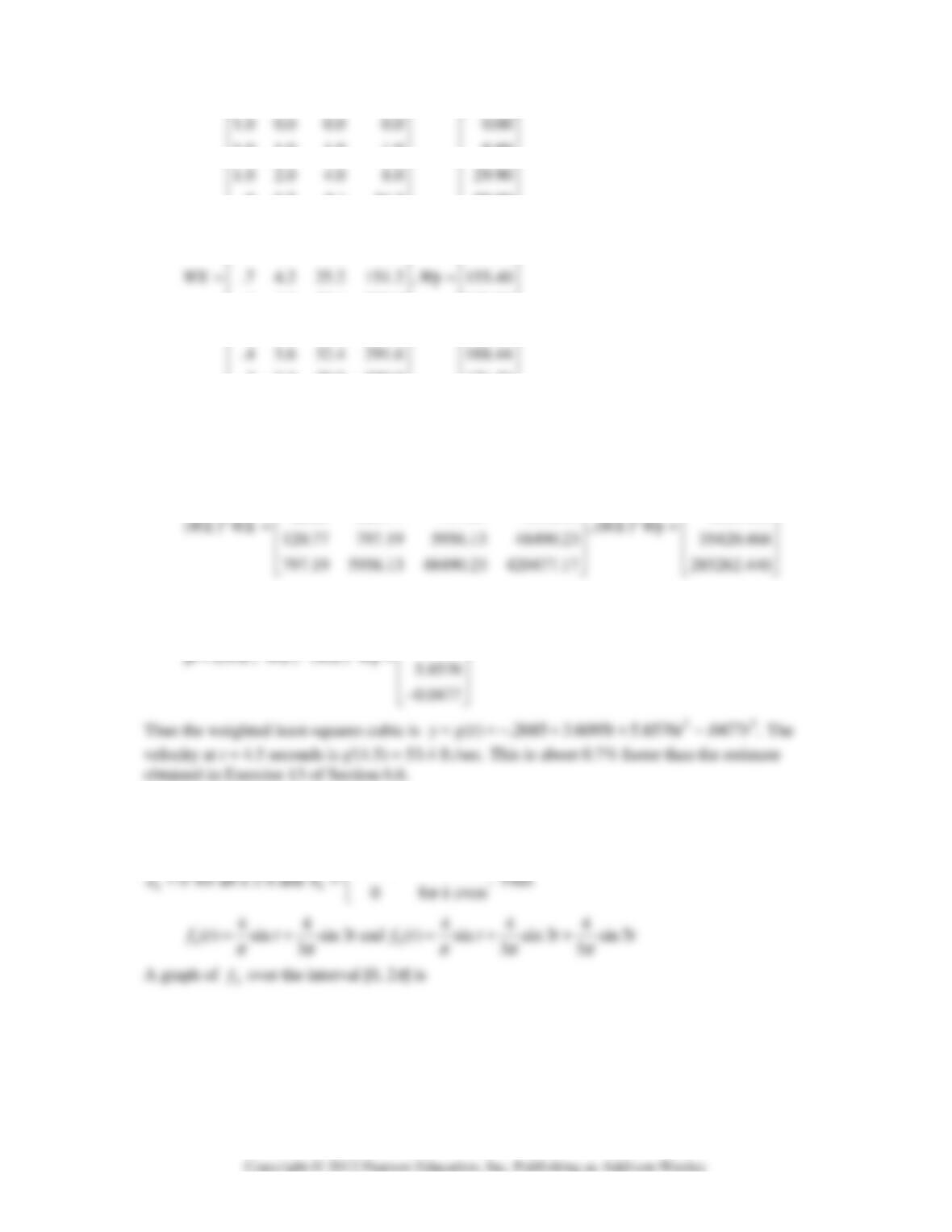
15. [M] The weighting matrix W is the 13 × 13 diagonal matrix with diagonal entries 1, 1, 1, .9, .9, .8, .7,
.6, .5, .4, .3, .2, .1. The design matrix X, parameter vector
β
, and observation vector y are:
⎢
⎢
⎢
⎢
23
23 0
23 1
2
23
3
⎢
⎢
23
23
23
⎢
⎣
10 0 0 0.0
144 4 104.7
155 5 159.1
166 6
,,
222.0
294.5
177 7
199 9
11010 10
11111 11
X
β
β
β
β
⎡⎤
⎢⎥
⎢⎥
⎢⎥
⎢⎥
⎡⎤
⎢⎥
⎢⎥
⎢⎥
⎢⎥
===
⎢⎥
⎢⎥
⎢⎥
⎢⎥
⎢⎥
⎢⎥
⎣⎦
⎢⎥
⎢⎥
⎢⎥
⎢⎥
y
β
471.1
571.7
686.8
⎡
⎤
⎢
⎥
⎢
⎥
⎢
⎥
⎢
⎥
⎢
⎥
⎢
⎥
⎢
⎥
⎢
⎥
⎢
⎥
⎢
⎥
⎢
⎥
⎢
⎥
6.8 • Solutions 399
⎥
⎥
⎡
1.0 1.0 1.0 1.0
⎥
⎥
.9 2.7 8.1 24.3
.9 3.6 14.4 57.6
.8 4.0 20.0 100.0
.6 4.2 29.4 205.8
.5 4.0 32.0 256.0
⎥
⎥
.3 3.0 30.0 300.0
.2 2.2 24.2 266.2
.1 1.2 14.4 172.8
⎢
⎢
⎢
⎢
⎢
⎢
⎢
⎢
⎢
⎢
⎢
⎢
⎢
⎣⎦
8.80
55.80
94.23
127.28
176.70
190.20
171.51
137.36
80.92
⎢
⎥
⎥
⎢⎥
⎥
⎢⎥
⎥
⎢⎥
⎥
⎢⎥
⎥
⎢⎥
⎥
⎢⎥
⎥
⎢⎥
⎥
⎢⎥
⎥
⎢⎥
⎥
⎢⎥
⎥
⎢⎥
⎥
⎢⎥
⎣
⎦
Further compute
6.66 22.23 120.77 797.19 747.844
22.23 120.77 797.19 5956.13 4815.438
⎡⎤⎡⎤
⎢⎥⎢⎥
and find that
1
0.2685
3.6095
ˆ(( ) ) ( ) 5.8576
TT
−
−
⎡⎤
⎢⎥
⎢⎥
16. [M] Let 1for0
() .
1for 2
t
ft t
π
ππ
≤<
⎧
=⎨−≤<
⎩ The Fourier coefficients for f have already been found to be
kk
π
⎧
400 CHAPTER 6 • Orthogonality and Least Squares
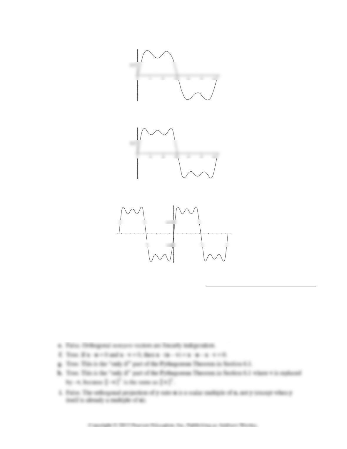
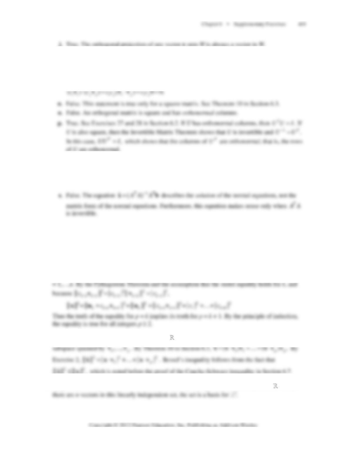
A graph of
5
f
over the interval [0, 2
π
] is
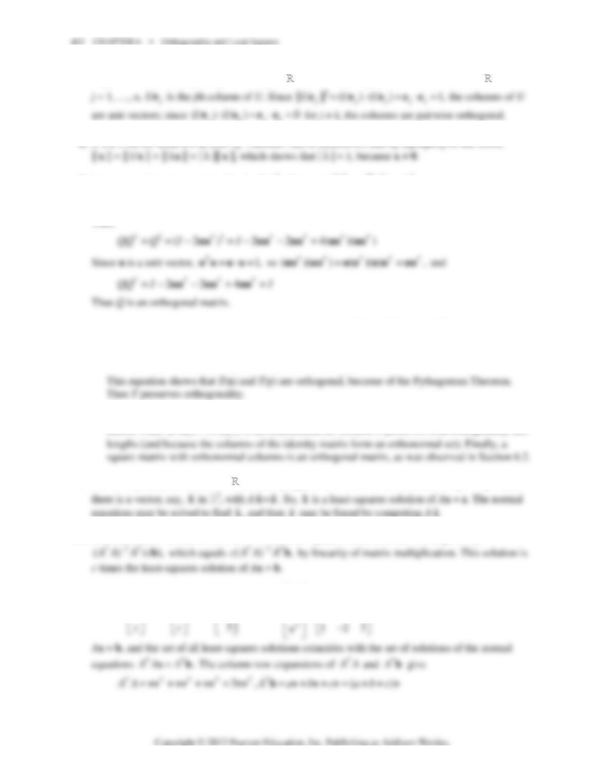
A graph of
5
f
over the interval [–2
π
, 2
π
] is
Chapter 6 SUPPLEMENTARY EXERCISES
1. a. False. The length of the zero vector is zero.
b. True. By the displayed equation before Example 2 in Section 6.1, with c = –1,
|| –x || = || (–1)x || =| –1 ||| x || = || x ||.
c. True. This is the definition of distance.
d. False. This equation would be true if r|| v || were replaced by | r ||| v ||.
1
–0.5
–1
1
–0.5
–1
1
–1
–6 –4 –2 246
k. True. This is a special case of the statement in the box following Example 6 in Section 6.1 (and
proved in Exercise 30 of Section 6.1).
l. False. The zero vector is in both W and
.W
⊥
m. True. See Exercise 32 in Section 6.2. If
0,
ij
⋅=vv
then
q. True. By the Orthogonal Decomposition Theorem, the vectors
proj
Wv
and
proj
W
−
vv
are
orthogonal, so the stated equality follows from the Pythagorean Theorem.
r. False. A least-squares solution is a vector
ˆ
x
(not A
ˆ
x
) such that A
ˆ
x
is the closest point to b
in Col A.
2. If
12
{, }
vv
is an orthonormal set and
11 2 2
,cc=+
xv v
then the vectors
11
c
v
and
22
c
v
are orthogonal
(Exercise 32 in Section 6.2). By the Pythagorean Theorem and properties of the norm
22222222
11 2 2 11 2 2 1 1 2 2 1 2
|| || || || || || || || ( || ||) ( || ||) | | | |cc c c c c c c=+ = + = + =+xvv v v v v
So the stated equality holds for p = 2. Now suppose the equality holds for p = k, with k ≥ 2. Let
11
{, , }
k
+
…
vv
be an orthonormal set, and consider
11 1 1 1 1
,
kk k k k k k
ccc c
++ ++
=+…+ + =+
xv v v u v
where
11
.
kkk
cc=+…+
uv v
Observe that
k
u
and
11
kk
c
++
v
are orthogonal because
1
0
jk+
⋅=vv
for j
3. Given x and an orthonormal set
1
{, , }
p
…vv
in
n
, let
ˆ
x
be the orthogonal projection of x onto the
4. By parts (a) and (c) of Theorem 7 in Section 6.2,
1
{,, }
k
UU…
vv
is an orthonormal set in
n
. Since
5. Suppose that (U x)⋅(U y) = x⋅y for all x, y in
n
, and let
1
,,
n
…
ee
be the standard basis for
n
. For
7. Let u be a unit vector, and let
2.
T
QI=−uu
Since
() ,
TT TT T T
==uu u u uu
(2 ) 2( ) 2
TTTTTT
QI I I Q= − =− =− =uu uu uu
Then
8. a. Suppose that x ⋅ y = 0. By the Pythagorean Theorem,
22 2
|| || || || || || .+=+xyxy
Since T preserves
lengths and is linear,
22 2 2
|| ( ) || || ( ) || || ( ) || || ( ) ( ) ||TTT TT+=+=+xyxyxy
b . The standard matrix of T is
[]
1
() ( )
n
TT…ee
, where
1
,,
n
…
ee
are the columns of the identity
matrix. Then
{( ), , ( )}
TT…
ee
is an orthonormal set because T preserves both orthogonality and
9. Let W = Span{u, v}. Given z in
n
, let
ˆproj .
W
=
zz
Then
ˆ
z
is in Col A, where
[]
.A=uv
Thus
x
z
10. Use Theorem 14 in Section 6.5. If c ≠ 0, the least-squares solution of Ax = c
b is given by
11. Let
,
x
y
⎢
⎣
⎡⎤
⎢⎥
=⎢⎥
x
,
a
b
⎡⎤
⎢⎥
=⎢⎥
b
1
2,
⎡⎤
⎢⎥
=−
⎢⎥
v
and
125
125.
T
T
A
⎡⎤ −
⎡
⎤
⎢⎥
⎢
⎥
==−
⎢⎥
⎢
⎥
v
v
Then the given set of equations is
12. The equation (1) in the exercise has been written as Vλ = b, where V is a single nonzero column
vector v, and b = Av. The least-squares solution
ˆ
λ
of Vλ = b is the exact solution of the normal
13. a. The row-column calculation of Au shows that each row of A is orthogonal to every u in Nul A. So
each row of A is in
(Nul ) .A
⊥
Since
(Nul )A
⊥
is a subspace, it must contain all linear
combinations of the rows of A; hence
(Nul )A
⊥
contains Row A.
14. The equation Ax = b has a solution if and only if b is in Col A. By Exercise 13(c), Ax = b has a
15. If
T
AURU=
with U orthogonal, then A is similar to R (because U is invertible and
1
T
UU
−
=
), so A
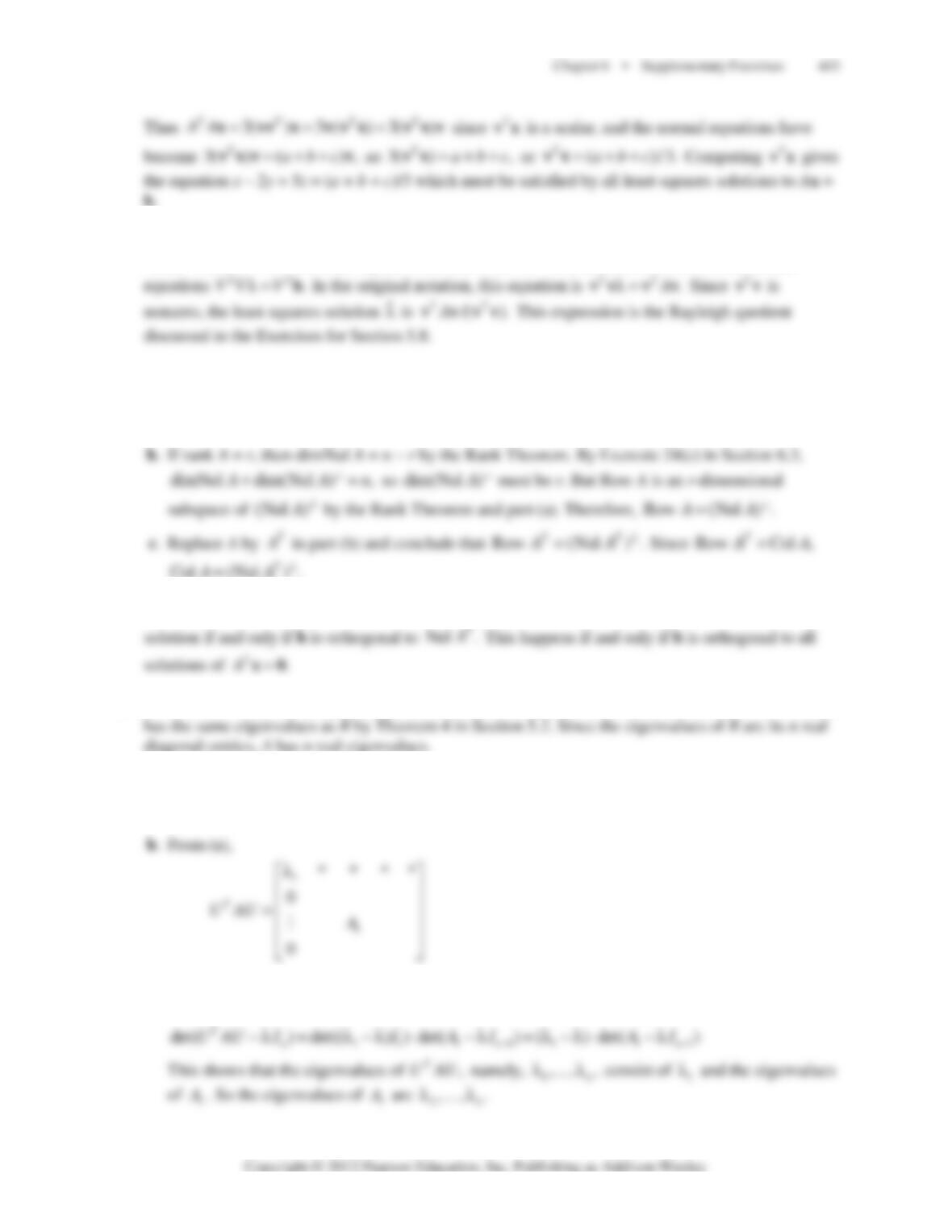
16. a. If
[]
12
,
n
U=…uu u
then
[]
11 2
.
n
AU A A=λ …uu u
Since
1
u
is a unit vector and
2
,,
n
…
uu
are orthogonal to
1
,
u
the first column of
T
UAU
is
11 1 1 11
() .
TT
UUλ=λ =λuue
View
T
UAU
as a 2 × 2 block upper triangular matrix, with
1
A
as the (2, 2)-block. Then from
Supplementary Exercise 12 in Chapter 5,
404 CHAPTER 6 • Orthogonality and Least Squares
17. [M] Compute that || Δx ||/|| x || = .4618 and
4
cond( ) (|| || / || ||) 3363 (1.548 10 ) .5206A
−
×=××=bbΔ
. In
18. [M] Compute that || Δx ||/|| x || = .00212 and cond(A) × (|| Δb ||/|| b ||) = 3363 × (.00212) ≈ 7.130. In
19. [M] Compute that
8
|| || / || || 7.178 10
−
=×xxΔ
and
4
cond( ) (|| || / || ||) 23683 (2.832 10 )A
−
×=××=bbΔ
6.707.
Observe that the relative change in x is much smaller than the relative change in b. In fact the
20. [M] Compute that || Δx ||/|| x || = .2597 and
5
cond( ) (|| || / || ||) 23683 (1.097 10 ) .2598A
−
×=××=bbΔ
.