5.7 • Solutions 333
where
1
c and
2
c are arbitrary complex numbers. To build the general real solution, rewrite
(3 )it
ev
as:
(3 ) 33(cos3 sin 3 )
2
it i
etit
−+
⎡⎤
=+
⎢⎥
⎣⎦
v
The general real solution has the form
3cos3 3sin3 3sin3 3cos3
tt t t
−− −+
⎡⎤⎡⎤
12. 710
.
45
−
⎡⎤
=⎢⎥
−
⎣⎦
A An eigenvalue of A is
12i−+
with corresponding eigenvector 3.
2
−
⎡⎤
=⎢⎥
⎣⎦
v
i
The
complex eigenfunctions
t
ev and
t
ev
form a basis for the set of all complex solutions to
.A′=xx
where
1
c and
2
c are arbitrary complex numbers. To build the general real solution, rewrite
(12)it
e
−+
v
as:
(12) 3(cos 2 sin 2 )
2
it t
i
eetit
−+ −
−
⎡⎤
=+
⎢⎥
⎣⎦
v
The general real solution has the form
12
3cos2 sin 2 3sin2 cos2
2cos2 2sin2
tt
tt t t
cec e
tt
−−
+−
⎡⎤⎡⎤
+
⎢⎥⎢⎥
⎣⎦⎣⎦
13. 43
.
62
−
⎡⎤
=⎢⎥
−
⎣⎦
A An eigenvalue of A is
13i+
with corresponding eigenvector 1.
2
+
⎡⎤
=⎢⎥
⎣⎦
v
i
The
complex eigenfunctions
t
ev and
t
ev
form a basis for the set of all complex solutions to
.A′=xx
The general complex solution is
334 CHAPTER 5 • Eigenvalues and Eigenvectors
where
1
c and
2
c are arbitrary complex numbers. To build the general real solution, rewrite
(1 3 )it
e
+
v
as:
(1 3 ) 1(cos 3 sin 3 )
2
it t
i
eetit
++
⎡⎤
=+
⎢⎥
⎣⎦
v
The general real solution has the form
12
cos 3 sin 3 sin 3 cos 3
2cos3 2sin3
tt
tt t t
cec e
tt
−+
⎡⎤⎡⎤
+
⎢⎥⎢⎥
⎣⎦⎣⎦
14. 21
.
82
−
⎡⎤
=⎢⎥
−
⎣⎦
A An eigenvalue of A is 2i with corresponding eigenvector 1.
4
−
⎡⎤
=⎢⎥
⎣⎦
v
i
The complex
eigenfunctions
t
ev and
t
ev
form a basis for the set of all complex solutions to
.A′=xx
The
general complex solution is
where
1
c and
2
c are arbitrary complex numbers. To build the general real solution, rewrite
(2 )it
ev
as:
(2 ) 1(cos 2 sin 2 )
4
it i
etit
−
⎡⎤
=+
⎢⎥
⎣⎦
v
The general real solution has the form
cos 2 sin 2 sin 2 cos 2
tt t t
+−
⎡⎤⎡⎤
15. [M]
8126
212.
7125
−− −
⎡⎤
⎢⎥
=⎢⎥
⎢⎥
⎣⎦
A
The eigenvalues of A are:
-1.0000
1.0000
nulbasis(A-ev(2)*eye(3))
=
-1.2000
1.0000
6
−
⎡⎤
nulbasis (A-ev(3)*eye(3))
=
-1.0000
so that
3
1
0
1
−
⎡⎤
⎢⎥
=⎢⎥
⎢⎥
⎣⎦
v
336 CHAPTER 5 • Eigenvalues and Eigenvectors
16. [M]
61116
254.
4510
−−
⎡⎤
⎢⎥
=−
⎢⎥
⎢⎥
−−
⎣⎦
A
The eigenvalues of A are:
ev = eig(A)=
4.0000
nulbasis(A-ev(1)*eye(3))
=
2.3333
7
⎡⎤
nulbasis(A-ev(2)*eye(3))
=
3.0000
so that
2
3
1
1
⎡⎤
⎢⎥
=−
⎢⎥
⎢⎥
⎣⎦
v
nulbasis(A-ev(3)*eye(3))
=
2.0000
so that
3
2
0
1
⎡⎤
⎢⎥
=⎢⎥
⎢⎥
⎣⎦
v
5.7 • Solutions 337
17. [M]
30 64 23
11 23 9 .
6154
⎡⎤
⎢⎥
=− − −
⎢⎥
⎢⎥
⎣⎦
A
The eigenvalues of A are:
ev = eig(A)=
5.0000 + 2.0000i
1.0000
nulbasis(A-ev(1)*eye(3))
=
so that
1
23 34
914
i
i
−
⎡⎤
⎢⎥
=−+
⎢⎥
v
nulbasis (A-ev(2)*eye(3))
=
7.6667 + 11.3333i
23 34
i
+
⎡⎤
nulbasis (A-ev(3)*eye(3))
=
-3.0000
3
−
⎡⎤
Hence the general complex solution is
23 34 23 34 3
ii
−+−
⎡⎤ ⎡⎤ ⎡⎤
Rewriting the first eigenfunction yields
555
23 34 23cos 2 34sin 2 23sin 2 34cos 2
9 14 (cos 2 sin 2 ) 9 cos 2 14sin 2 9sin 2 14 cos 2
ttt
itttt
ie t i t t te i t te
−+−
⎡⎤ ⎡ ⎤⎡ ⎤
⎢⎥ ⎢ ⎥⎢ ⎥
−+ + =− − + − +
⎢⎥ ⎢ ⎥⎢ ⎥
338 CHAPTER 5 • Eigenvalues and Eigenvectors
23cos 2 34sin 2 23sin 2 34 cos 2 3
tt t t
+−−
⎡⎤⎡⎤⎡⎤
where
12
,,cc and
3
c are real. The origin is a repellor, because the real parts of all eigenvalues are
positive. All trajectories spiral away from the origin.
18. [M]
53 30 2
90 52 3 .
A
−−
⎡⎤
⎢⎥
=−−
⎢⎥
The eigenvalues of A are:
-7.0000
nulbasis(A-ev(1)*eye(3))
=
0.5000
1
⎡⎤
⎣⎦
nulbasis(A-ev(2)*eye(3))
=
0.6000 + 0.2000i
62
i
+
⎡⎤
nulbasis(A-ev(3)*eye(3))
=
0.6000 – 0.2000i
62
i
−
⎡⎤
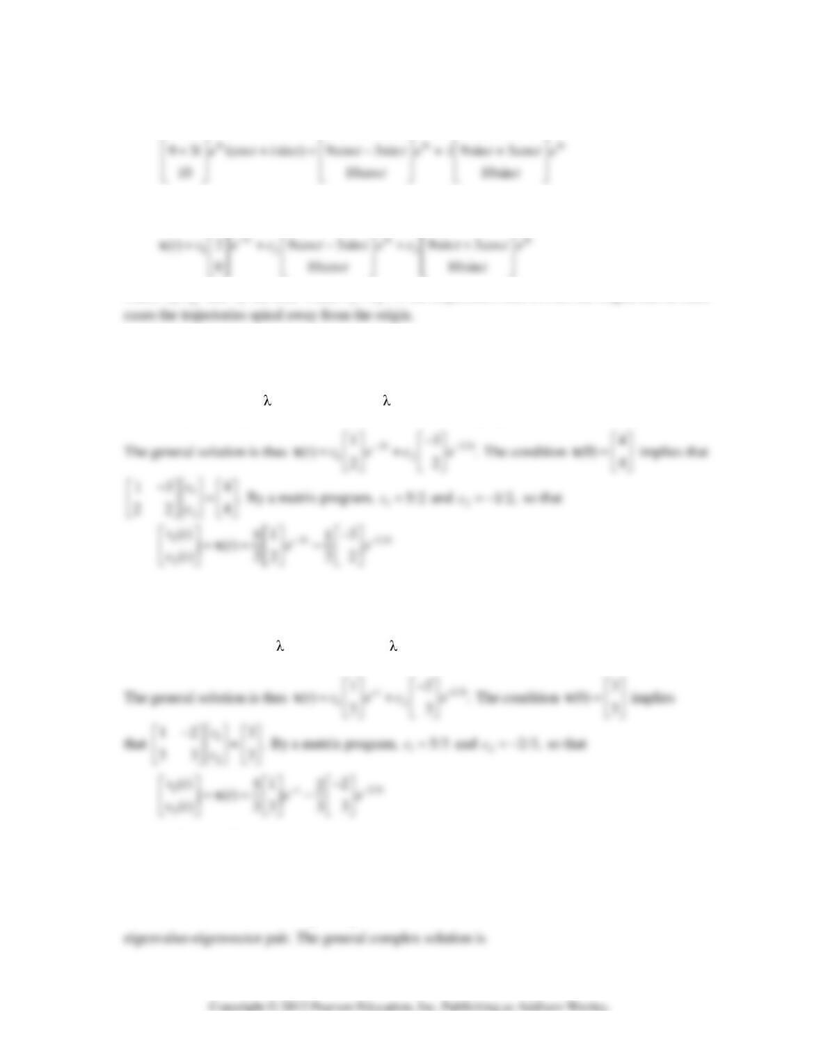
Hence the general complex solution is
162 62
ii
+−
⎡⎤ ⎡ ⎤ ⎡ ⎤
5.7 • Solutions 339
Rewriting the second eigenfunction yields
6 2 6cos 2sin 6sin 2cos
+−+
⎡⎤ ⎡ ⎤ ⎡ ⎤
itttt
Hence the general real solution is
1 6cos 2sin 6sin 2cos
tt t t
−+
⎡⎤ ⎡ ⎤ ⎡ ⎤
where
,,cc and
c are real. When
0cc==
the trajectories tend toward the origin, and in other
19. [M] Substitute
121
15 13 4,=/, =/, =RRC
and
2
3C= into the formula for A given in Example 1, and
use a matrix program to find the eigenvalues and eigenvectors:
11 2 1
234 1 3
525
11 2 2
A−/ −
⎡⎤ ⎡⎤ ⎡⎤
= , =−. : = , =− . : =
⎢⎥ ⎢⎥ ⎢⎥
−
⎣⎦ ⎣⎦ ⎣⎦
vv
20. [M] Substitute
121
115 13 9,RRC=/ , =/, = and
2
2C= into the formula for A given in Example 1,
and use a matrix program to find the eigenvalues and eigenvectors:
11 2 2
213 1 2
125
32 32 3 3
A−/ −
⎡⎤ ⎡⎤ ⎡⎤
=,=−:=,=−.:=
⎢⎥ ⎢⎥ ⎢⎥
/−/
⎣⎦ ⎣⎦ ⎣⎦
vv
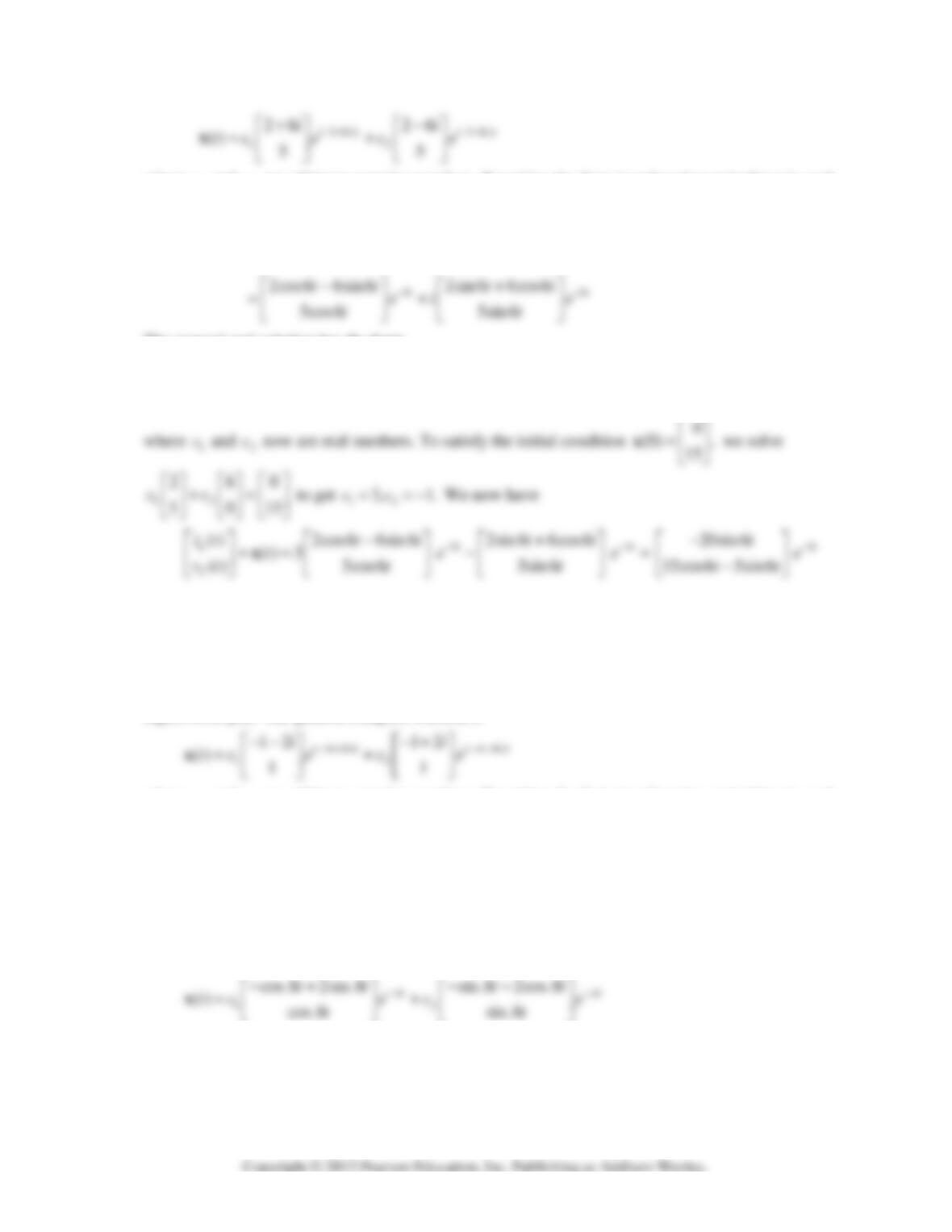
21. [M] 18
.
55
−−
⎡⎤
=⎢⎥
−
⎣⎦
A Using a matrix program we find that an eigenvalue of A is
36i−+
with
corresponding eigenvector 26.
5
+
⎡⎤
=⎢⎥
⎣⎦
v
i
The conjugates of these form the second
340 CHAPTER 5 • Eigenvalues and Eigenvectors
where
1
c and
2
c are arbitrary complex numbers. Rewriting the first eigenfunction and taking its real
and imaginary parts, we have
(36) 3
26 (cos 6 sin 6 )
5
−+ −
+
⎡⎤
=+
⎢⎥
⎣⎦
vit t
i
eetit
The general real solution has the form
33
12
2cos6 6sin6 2sin6 6cos6
() 5cos6 5sin6
tt
tt t t
tc e c e
tt
−−
−+
⎡⎤⎡⎤
=+
⎢⎥⎢⎥
⎣⎦⎣⎦
x
22. [M] 02
.
48
⎡⎤
=⎢⎥
−. −.
⎣⎦
A Using a matrix program we find that an eigenvalue of A is
48i−. + .
with
corresponding eigenvector 12.
1
−−
⎡⎤
=⎢⎥
⎣⎦
v
i
The conjugates of these form the second eigenvalue-
eigenvector pair. The general complex solution is
where
1
c and
2
c are arbitrary complex numbers. Rewriting the first eigenfunction and taking its real
and imaginary parts, we have
(48) 4
44
12 (cos 8 sin 8 )
1
cos 8 2sin 8 sin 8 2cos 8
cos 8 sin 8
it t
tt
i
eetit
tt t t
ei e
tt
−. +. −.
−. −.
−−
⎡⎤
=.+.
⎢⎥
⎣⎦
−.+ . −.− .
⎡⎤⎡⎤
=+
⎢⎥⎢⎥
..
⎣⎦⎣⎦
v
The general real solution has the form
5.8 • Solutions 341
where
1
c and
2
c now are real numbers. To satisfy the initial condition 0
(0) ,
12
⎡⎤
=⎢⎥
⎣⎦
x we solve
12
12 0
1012
cc
−−
⎡⎤⎡⎤ ⎡⎤
+=
⎢⎥⎢⎥ ⎢⎥
⎣⎦ ⎣⎦⎣⎦
to get
12
12 6.=,=−cc We now have
5.8 SOLUTIONS
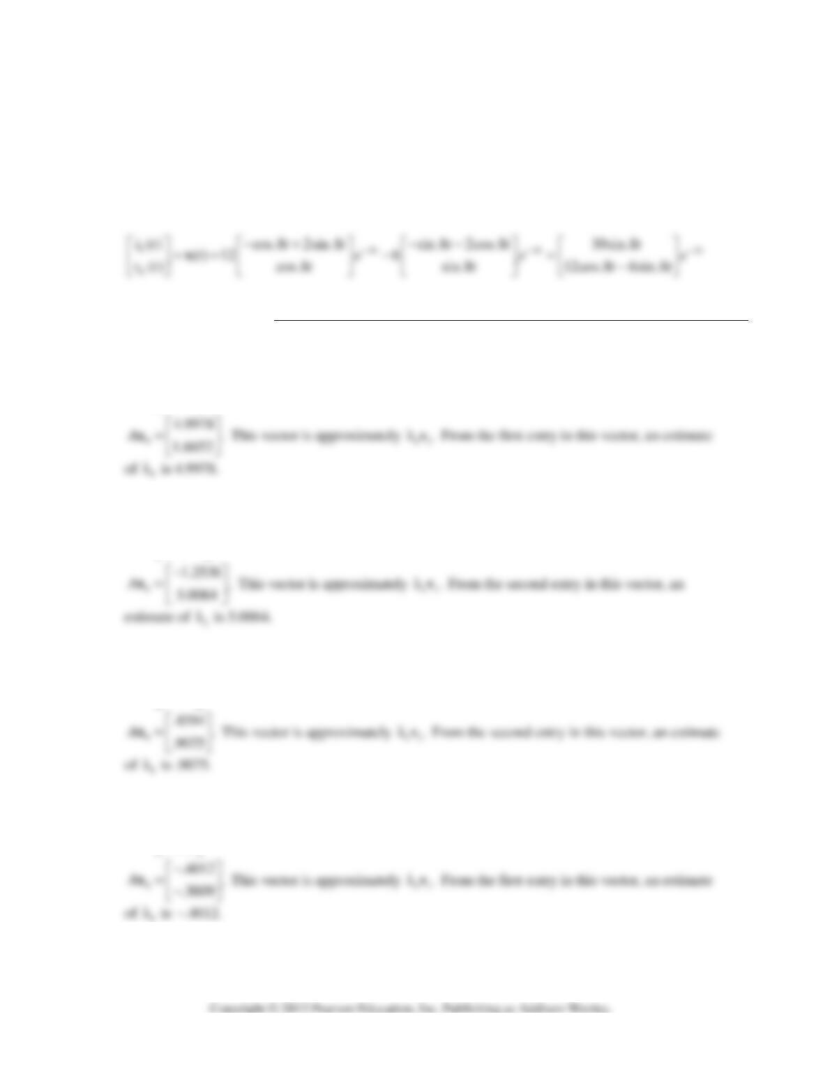
1. The vectors in the given sequence approach an eigenvector
1
.v The last vector in the sequence,
4
1,
3326
⎡⎤
=⎢⎥
.
⎣⎦
x is probably the best estimate for
1
.v To compute an estimate for
1
,λ examine
2. The vectors in the given sequence approach an eigenvector
1
.v The last vector in the sequence,
4
2520 ,
1
−.
⎡⎤
=⎢⎥
⎣⎦
x is probably the best estimate for
1
.v To compute an estimate for
1
,λ examine
3. The vectors in the given sequence approach an eigenvector
1
.v The last vector in the sequence,
4
5188 ,
1
.
⎡⎤
=⎢⎥
⎣⎦
x is probably the best estimate for
1
.v To compute an estimate for
1
,λ examine
4. The vectors in the given sequence approach an eigenvector
1
.v The last vector in the sequence,
4
1,
7502
⎡⎤
=⎢⎥
.
⎣⎦
x is probably the best estimate for
1
.v To compute an estimate for
1
,λ examine
342 CHAPTER 5 • Eigenvalues and Eigenvectors
5. Since
5
24991
31241
A⎡⎤
=⎢⎥
−
⎣⎦
x is an estimate for an eigenvector, the vector
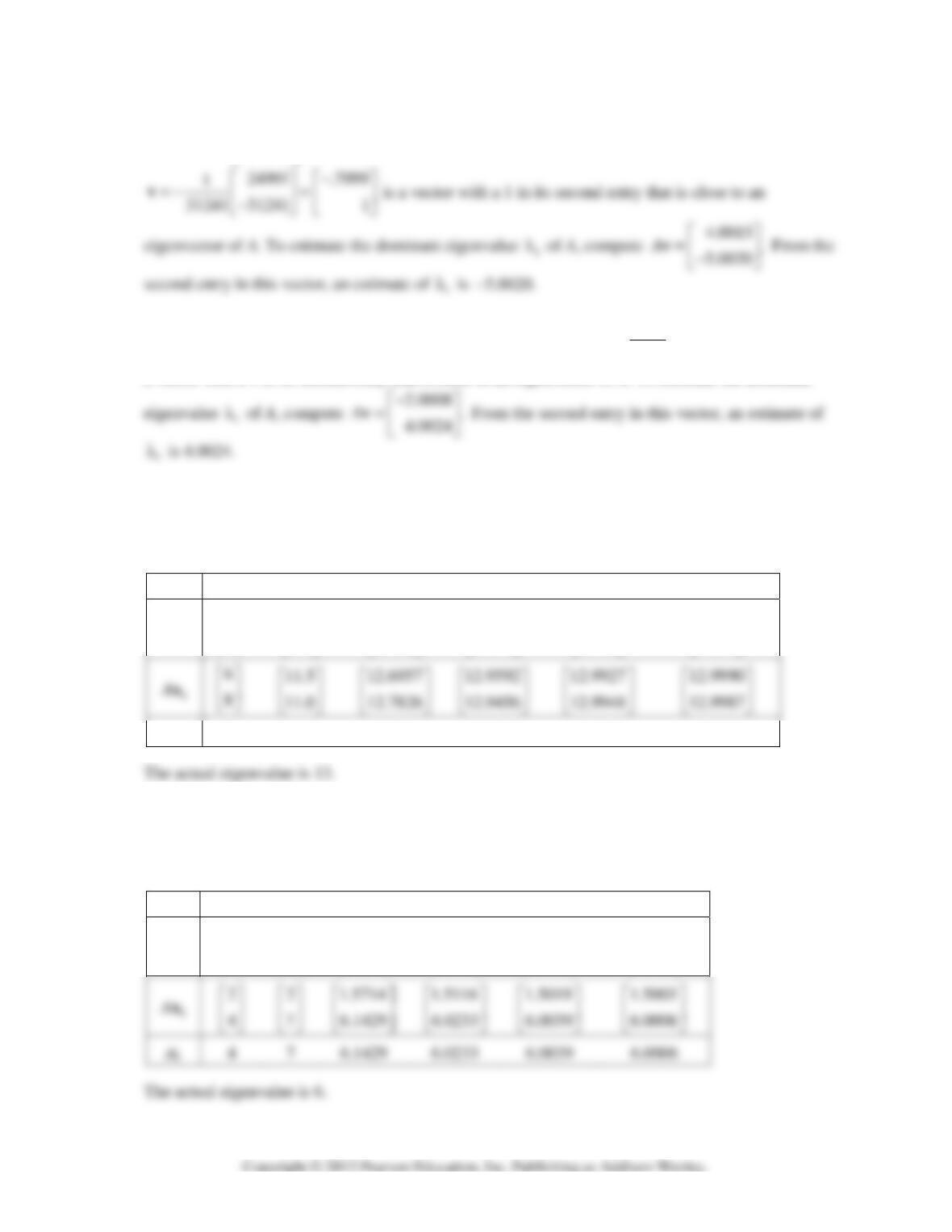
6. Since
5
2045
4093
A−
⎡⎤
=⎢⎥
⎣⎦
x is an estimate for an eigenvector, the vector 2045 4996
1
4093 1
4093
−−.
⎡⎤⎡ ⎤
==
⎢⎥⎢ ⎥
⎣⎦⎣ ⎦
v is
a vector with a 1 in its second entry that is close to an eigenvector of A. To estimate the dominant
7. [M]
0
67 1
.
85 0
⎡⎤ ⎡⎤
=,=
⎢⎥ ⎢⎥
⎣⎦ ⎣⎦
xA The data in the table below was calculated using Mathematica, which
carried more digits than shown here.
k 0 1 2 3 4 5
k
x 1
0
⎡⎤
⎢⎥
⎣⎦
75
1
.
⎡⎤
⎢⎥
⎣⎦
1
9565
⎡⎤
⎢⎥
.
⎣⎦
9932
1
.
⎡
⎤
⎢
⎥
⎣
⎦ 1
9990
⎡
⎤
⎢
⎥
.
⎣
⎦ .9998
1
⎡⎤
⎢⎥
⎣⎦
⎡
⎢
⎣
⎡
⎢
⎣
k
µ
8 11.5 12.7826 12.9592 12.9948 12.9990
8. [M]
0
21 1
.
45 0
⎡⎤ ⎡⎤
=,=
⎢⎥ ⎢⎥
⎣⎦ ⎣⎦
xA The data in the table below was calculated using Mathematica, which
carried more digits than shown here.
k 0 1 2 3 4 5
k
x 1
0
⎡⎤
⎢⎥
⎣⎦
5
1
.
⎡⎤
⎢⎥
⎣⎦
2857
1
.
⎡⎤
⎢⎥
⎣⎦
2558
1
.
⎡
⎤
⎢
⎥
⎣
⎦ 2510
1
.
⎡
⎤
⎢
⎥
⎣
⎦ .2502
1
⎡
⎤
⎢
⎥
⎣
⎦
⎡
⎢
⎣
⎡
⎢
⎣
⎡
⎢
⎣
µ
5.8 • Solutions 343
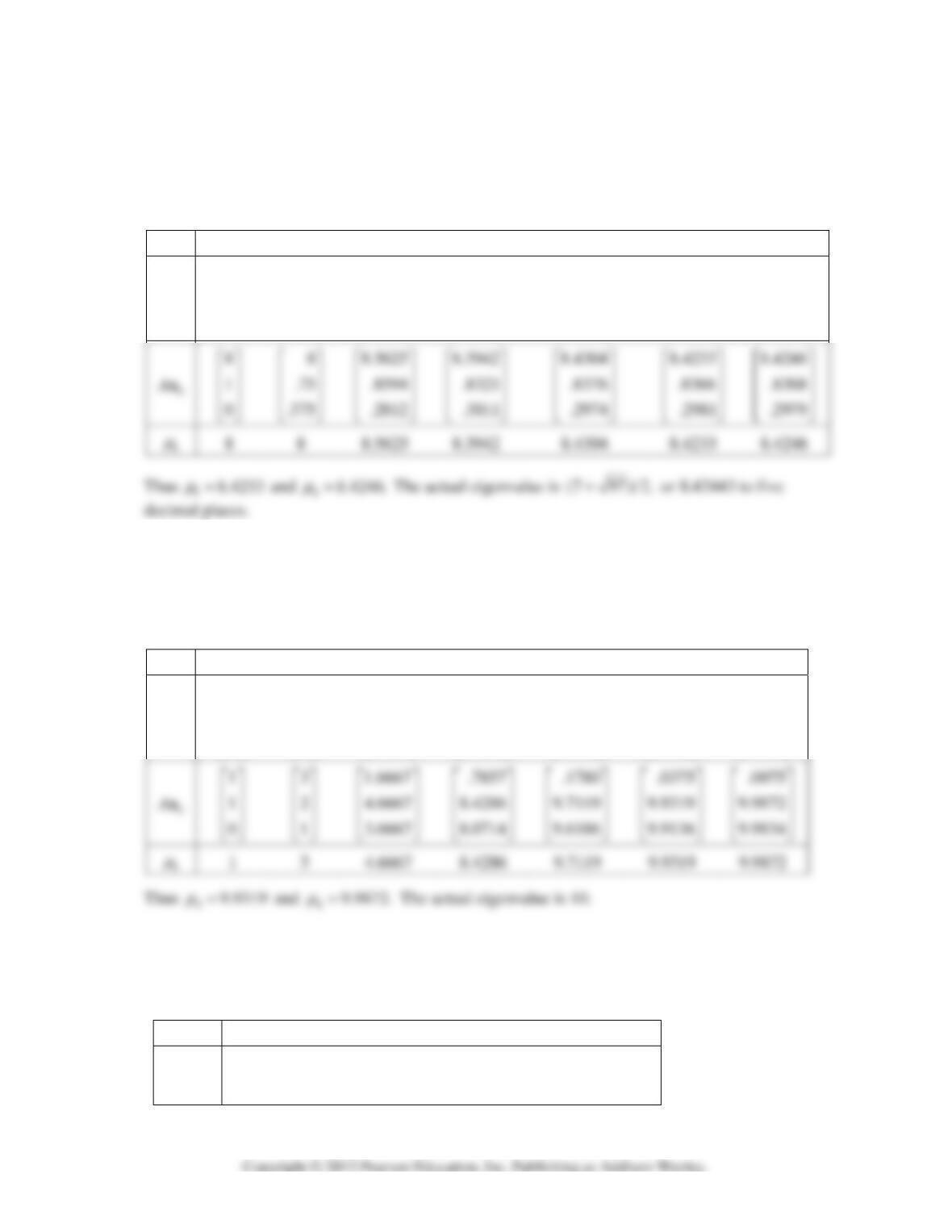
9. [M]
0
8012 1
121 0.
030 0
⎡⎤⎡⎤
⎢⎥⎢⎥
=− ,=
⎢⎥⎢⎥
⎢⎥⎢⎥
⎣⎦⎣⎦
xA
The data in the table below was calculated using Mathematica,
which carried more digits than shown here.
k 0 1 2 3 4 5 6
k
x
1
0
0
⎡⎤
⎢⎥
⎢⎥
⎢⎥
⎣⎦
1
125
0
⎡⎤
⎢⎥
.
⎢⎥
⎢⎥
⎣⎦
1
0938
0469
⎡⎤
⎢⎥
.
⎢⎥
⎢⎥
.
⎣⎦
1
1004
0328
⎡
⎤
⎢
⎥
.
⎢
⎥
⎢
⎥
.
⎣
⎦
1
0991
0359
⎡
⎤
⎢
⎥
.
⎢
⎥
⎢
⎥
.
⎣
⎦
1
0994
0353
⎡⎤
⎢⎥
.
⎢⎥
⎢⎥
.
⎣⎦
1
0993
0354
⎡⎤
⎢⎥
.
⎢⎥
⎢⎥
.
⎣⎦
⎡
⎢
⎢
⎢
⎣
⎡
⎢
⎢
⎢
⎣
⎡
⎢
⎢
⎢
⎣
10. [M]
0
12 2 1
11 9 0.
01 9 0
−
⎡⎤⎡⎤
⎢⎥⎢⎥
=,=
⎢⎥⎢⎥
⎢⎥⎢⎥
⎣⎦⎣⎦
xA
The data in the table below was calculated using Mathematica,
which carried more digits than shown here.
k 0 1 2 3 4 5 6
k
x
1
0
0
⎡⎤
⎢⎥
⎢⎥
⎢⎥
⎣⎦
1
1
0
⎡
⎤
⎢
⎥
⎢
⎥
⎢
⎥
⎣
⎦
1
6667
3333
⎡⎤
⎢⎥
.
⎢⎥
⎢⎥
.
⎣⎦
3571
1
7857
.
⎡
⎤
⎢
⎥
⎢
⎥
⎢
⎥
.
⎣
⎦
0932
1
9576
.
⎡
⎤
⎢
⎥
⎢
⎥
⎢
⎥
.
⎣
⎦
0183
1
9904
.
⎡
⎤
⎢
⎥
⎢
⎥
⎢
⎥
.
⎣
⎦
0038
1
9982
.
⎡⎤
⎢⎥
⎢⎥
⎢⎥
.
⎣⎦
⎡
⎢
⎢
⎢
⎣
⎡
⎢
⎢
⎢
⎣
⎡
⎢
⎢
⎢
⎣
⎡
⎢
⎢
⎢
⎣
11. [M]
0
52 1
.
22 0
⎡⎤ ⎡⎤
=,=
⎢⎥ ⎢⎥
⎣⎦ ⎣⎦
xA The data in the table below was calculated using Mathematica, which
carried more digits than shown here.
k 0 1 2 3 4
k
x 1
0
⎡⎤
⎢⎥
⎣⎦
1
4
⎡⎤
⎢⎥
.
⎣⎦
1
4828
⎡
⎤
⎢
⎥
.
⎣
⎦ 1
4971
⎡
⎤
⎢
⎥
.
⎣
⎦ 1
4995
⎡
⎤
⎢
⎥
.
⎣
⎦
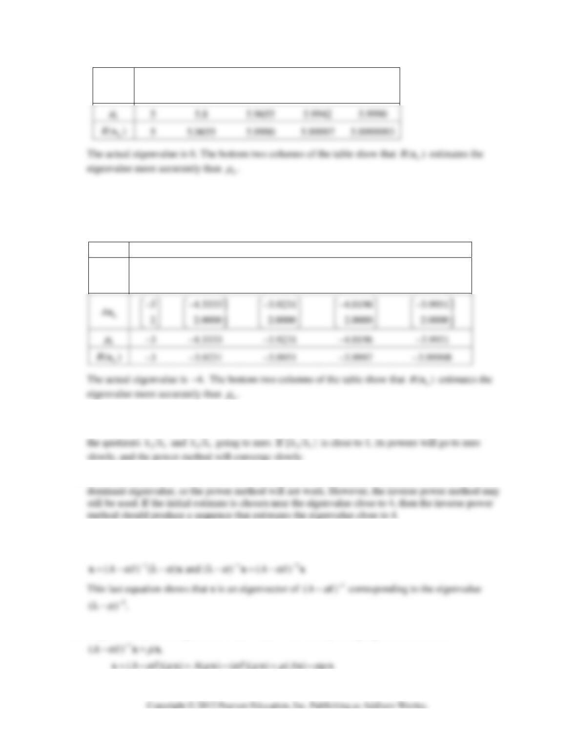
344 CHAPTER 5 • Eigenvalues and Eigenvectors
k
Ax 5
2
⎡⎤
⎢⎥
⎣⎦
58
28
.
⎡⎤
⎢⎥
.
⎣⎦
5 9655
2 9655
.
⎡⎤
⎢⎥
.
⎣⎦
59942
2 9942
.
⎡
⎤
⎢
⎥
.
⎣
⎦ 59990
2 9990
.
⎡
⎤
⎢
⎥
.
⎣
⎦
12. [M]
0
32 1
.
22 0
−
⎡⎤⎡⎤
=,=
⎢⎥⎢⎥
⎣⎦⎣⎦
xA The data in the table below was calculated using Mathematica,
which carried more digits than shown here.
k 0 1 2 3 4
k
x 1
0
⎡⎤
⎢⎥
⎣⎦
1
6667
⎡⎤
⎢⎥
−.
⎣⎦
1
4615
⎡
⎤
⎢
⎥
−.
⎣
⎦ 1
5098
⎡
⎤
⎢
⎥
−.
⎣
⎦ 1
4976
⎡⎤
⎢⎥
−.
⎣⎦
⎡
⎢
⎣
⎡
⎢
⎣
⎡
⎢
⎣
k
13. If the eigenvalues close to 4 and
4−
have different absolute values, then one of these is a strictly
dominant eigenvalue, so the power method will work. But the power method depends on powers of
14. If the eigenvalues close to 4 and
4−
have the same absolute value, then neither of these is a strictly
15. Suppose
,=λxxA
with
0.≠x
For any
().,− =λ−xx xAI
αα α
If
α
is not an eigenvalue of A, then
AI
α
−
is invertible and
α
λ−
is not 0; hence
16. Suppose that
µ
is an eigenvalue of
1
()AI
α
−
−
with corresponding eigenvector x. Since