5.8 • Solutions 345
Solving this equation for Ax, we find that
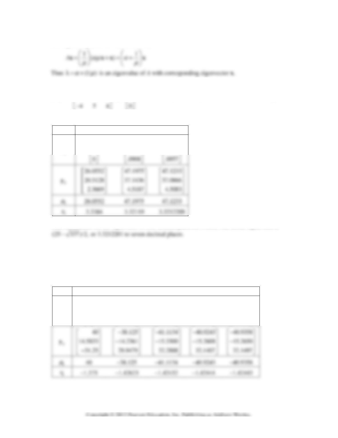
17. [M]
0
10 8 4 1
813 4 0 33.
−−
⎡⎤⎡⎤
⎢⎥⎢⎥
=− , = , =.
⎢⎥⎢⎥
⎣⎦⎣⎦
xA
α
The data in the table below was calculated using
Mathematica, which carried more digits than shown here.
k 0 1 2
k
x
1
0
⎢
⎢
⎣
⎡
⎢
⎢
⎢
⎣
⎡⎤
⎢⎥
1
7873
⎡⎤
⎢⎥
.
1
7870
⎡
⎤
⎢
⎥
.
Thus an estimate for the eigenvalue to four decimal places is 3.3212. The actual eigenvalue is
18. [M]
0
8012 1
121 0 14.
030 0
⎡⎤⎡⎤
⎢⎥⎢⎥
=− ,=,=−.
⎢⎥⎢⎥
⎢⎥⎢⎥
⎣⎦⎣⎦
xA
α
The data in the table below was calculated using
Mathematica, which carried more digits than shown here.
k 0 1 2 3 4
k
x
1
0
0
⎡⎤
⎢⎥
⎢⎥
⎢⎥
⎣⎦
1
3646
7813
⎡⎤
⎢⎥
.
⎢⎥
⎢⎥
−.
⎣⎦
1
3734
7855
⎡
⎤
⎢
⎥
.
⎢
⎥
⎢
⎥
−.
⎣
⎦
1
3729
7854
⎡
⎤
⎢
⎥
.
⎢
⎥
⎢
⎥
−.
⎣
⎦
1
3729
7854
⎡
⎤
⎢
⎥
.
⎢
⎥
⎢
⎥
−.
⎣
⎦
⎡
⎢
⎢
⎢
⎣
⎡
⎢
⎢
⎢
⎣
⎡
⎢
⎢
⎢
⎣
346 CHAPTER 5 • Eigenvalues and Eigenvectors
19. [M]
0
10 7 8 7 1
756 5 0
.
86109 0
75910 0
⎡⎤⎡⎤
⎢⎥⎢⎥
⎢⎥⎢⎥
=,=
⎢⎥⎢⎥
⎢⎥⎢⎥
⎢⎥⎢⎥
⎣⎦⎣⎦
xA
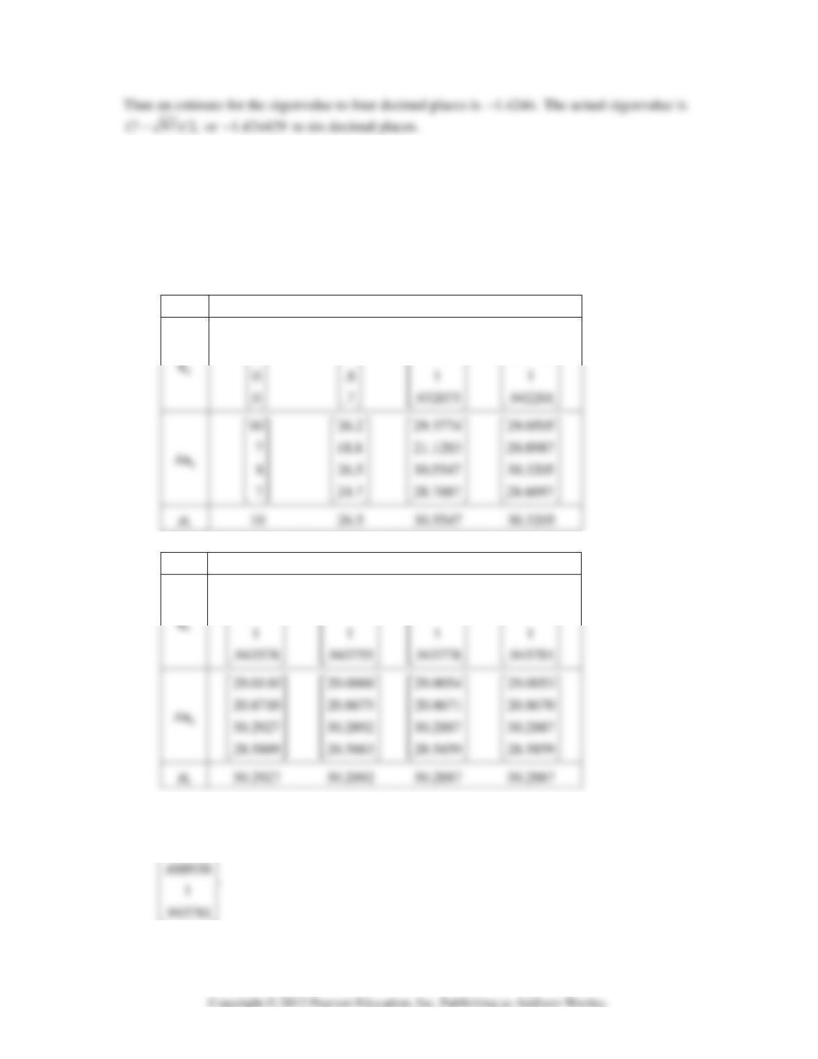
(a) The data in the table below was calculated using Mathematica, which carried more digits than
shown here.
k 0 1 2 3
⎢
⎢
⎢
⎢
⎣
⎢
⎢
⎢
⎢
⎣
⎢
⎢
⎢
⎢
⎣
⎡
⎢
⎢
⎢
⎢
⎢
⎣
⎡
⎢
⎢
⎢
⎢
⎢
⎣
1
0
⎡
⎤
⎢
⎥
1
7
⎡⎤
⎢⎥
.
988679
709434
.
⎡
⎤
⎢
⎥
.
961467
691491
.
⎡
⎤
⎢
⎥
.
k 4 5 6 7
⎢
⎢
⎢
⎣
⎢
⎢
⎢
⎣
⎡
⎢
⎢
⎢
⎢
⎢
⎣
⎡
⎢
⎢
⎢
⎢
⎢
⎣
958115
689261
.
⎡⎤
⎢⎥
.
⎢⎥
957691
688978
.
⎡⎤
⎢⎥
.
⎢⎥
957637
688942
.
⎡
⎤
⎢
⎥
.
⎢
⎥
957630
688938
.
⎡
⎤
⎢
⎥
.
⎢
⎥
Thus an estimate for the eigenvalue to four decimal places is 30.2887. The actual eigenvalue is
30.2886853 to seven decimal places. An estimate for the corresponding eigenvector is
957630
.
⎡⎤
5.8 • Solutions 347
(b) The data in the table below was calculated using Mathematica, which carried more digits than
shown here.
k 0 1 2 3 4
k
x
1
0
0
0
⎡⎤
⎢⎥
⎢⎥
⎢⎥
⎢⎥
⎢⎥
⎣⎦
609756
1
243902
146341
−.
⎡⎤
⎢⎥
⎢⎥
⎢⎥
−.
⎢⎥
.
⎢⎥
⎣⎦
604007
1
251051
148899
−.
⎡
⎤
⎢
⎥
⎢
⎥
⎢
⎥
−.
⎢
⎥
.
⎢
⎥
⎣
⎦
603973
1
251134
148953
−.
⎡
⎤
⎢
⎥
⎢
⎥
⎢
⎥
−.
⎢
⎥
.
⎢
⎥
⎣
⎦
603972
1
251135
148953
−.
⎡
⎤
⎢
⎥
⎢
⎥
⎢
⎥
−.
⎢
⎥
.
⎢
⎥
⎣
⎦
⎢
⎢
⎢
⎢
⎢
⎣
⎢
⎢
⎢
⎢
⎢
⎣
⎢
⎢
⎢
⎢
⎢
⎣
25
⎡⎤
59 5610
−.
⎡⎤
59 5041
−.
⎡
⎤
59 5044
−.
⎡
⎤
59 5044
−.
⎡
⎤
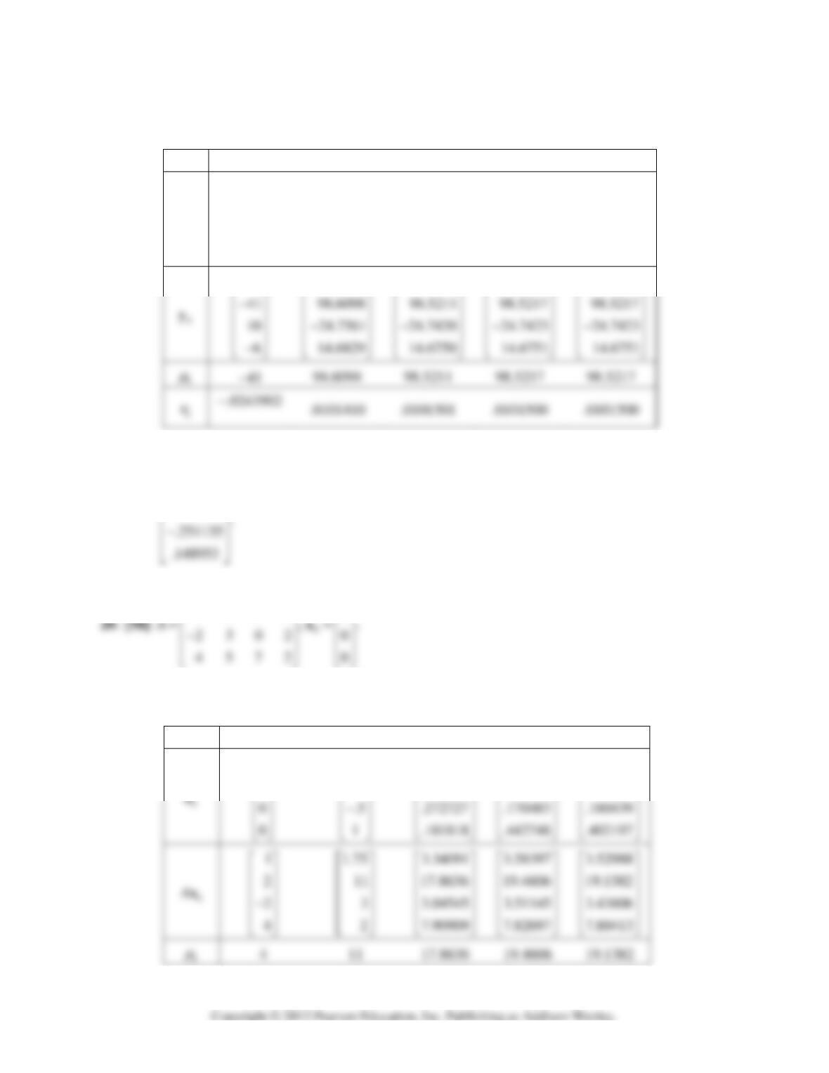
Thus an estimate for the eigenvalue to five decimal places is .01015. The actual eigenvalue is
.01015005 to eight decimal places. An estimate for the corresponding eigenvector is
603972
1.
−.
⎡⎤
⎢⎥
⎢⎥
1232 1
2121311 0
⎡⎤⎡⎤
⎢⎥⎢⎥
(a) The data in the table below was calculated using Mathematica, which carried more digits than
shown here.
k 0 1 2 3 4
⎢
⎢
⎢
⎣
⎢
⎢
⎢
⎣
⎢
⎢
⎢
⎣
⎢
⎢
⎢
⎣
⎡
⎢
⎢
⎢
⎢
⎢
⎣
⎡
⎢
⎢
⎢
⎢
⎢
⎣
⎡
⎢
⎢
⎢
⎢
⎢
⎣
⎡
⎢
⎢
⎢
⎢
⎢
⎣
1
0
⎡
⎤
⎢
⎥
⎢
⎥
25
5
.
⎡⎤
⎢⎥
.
⎢⎥
159091
1
.
⎡
⎤
⎢
⎥
⎢
⎥
187023
1
.
⎡
⎤
⎢
⎥
⎢
⎥
184166
1
.
⎡
⎤
⎢
⎥
⎢
⎥
348 CHAPTER 5 • Eigenvalues and Eigenvectors
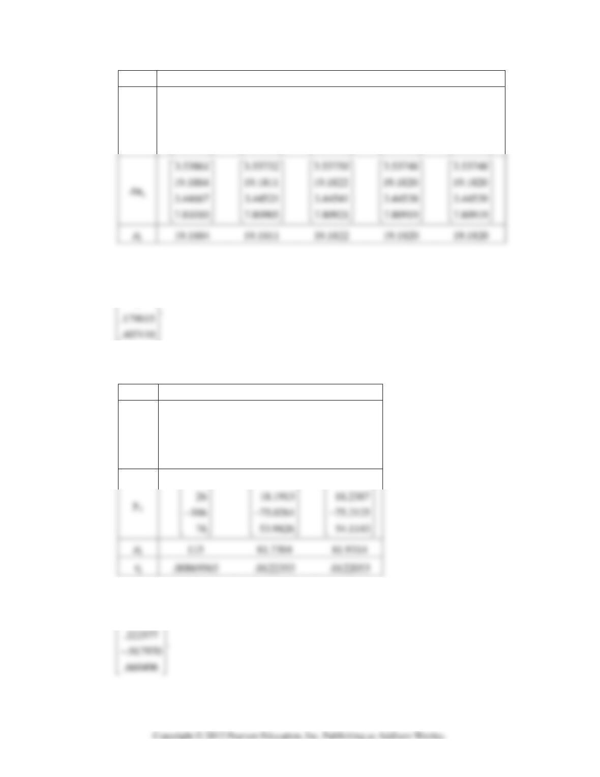
k 5 6 7 8 9
k
x
184441
1
179539
407778
.
⎡⎤
⎢⎥
⎢⎥
⎢⎥
.
⎢⎥
.
⎢⎥
⎣⎦
184414
1
179622
407021
.
⎡⎤
⎢⎥
⎢⎥
⎢⎥
.
⎢⎥
.
⎢⎥
⎣⎦
184417
1
179615
407121
.
⎡
⎤
⎢
⎥
⎢
⎥
⎢
⎥
.
⎢
⎥
.
⎢
⎥
⎣
⎦
184416
1
179615
407108
.
⎡
⎤
⎢
⎥
⎢
⎥
⎢
⎥
.
⎢
⎥
.
⎢
⎥
⎣
⎦
184416
1
179615
407110
.
⎡⎤
⎢⎥
⎢⎥
⎢⎥
.
⎢⎥
.
⎢⎥
⎣⎦
⎡
⎢
⎢
⎢
⎢
⎢
⎣
⎡
⎢
⎢
⎢
⎢
⎢
⎣
Thus an estimate for the eigenvalue to four decimal places is 19.1820. The actual eigenvalue is
19.1820368 to seven decimal places. An estimate for the corresponding eigenvector is
184416
1.
.
⎡⎤
⎢⎥
⎣⎦
(b) The data in the table below was calculated using Mathematica, which carried more digits than
shown here.
k 0 1 2
k
x
1
0
0
0
⎡
⎤
⎢
⎥
⎢
⎥
⎢
⎥
⎢
⎥
⎢
⎥
⎣
⎦
1
226087
921739
660870
⎡⎤
⎢⎥
.
⎢⎥
⎢⎥
−.
⎢⎥
.
⎢⎥
⎣⎦
1
222577
917970
660496
⎡
⎤
⎢
⎥
.
⎢
⎥
⎢
⎥
−.
⎢
⎥
.
⎢
⎥
⎣
⎦
⎢
⎢
⎢
⎢
⎢
⎣
⎢
⎢
⎢
⎢
⎢
⎣
115
⎡
⎤
81 7304
.
⎡⎤
81 9314
.
⎡
⎤
Thus an estimate for the eigenvalue to four decimal places is .0122. The actual eigenvalue is
.01220556 to eight decimal places. An estimate for the corresponding eigenvector is
1
⎡⎤
Chapter 5 • Supplementary Exercises 349
21. (a) 80 5
.
02 5
..
⎡⎤⎡⎤
=,=
⎢⎥⎢⎥
..
⎣⎦⎣⎦
xA Here is the sequence
k
Ax
for
15:=,k…
.. . . .
⎡⎤⎡ ⎤⎡ ⎤⎡ ⎤⎡ ⎤
(b) 10 5
.
08 5
.
⎡⎤⎡⎤
=,=
⎢⎥⎢⎥
..
⎣⎦⎣⎦
xA Here is the sequence
k
Ax
for
15:=,k…
.. . . .
⎡⎤⎡ ⎤⎡ ⎤⎡ ⎤⎡ ⎤
c. 80 5
.
02 5
.
⎡⎤⎡⎤
=,=
⎢⎥⎢⎥
.
⎣⎦⎣⎦
xA Here is the sequence
k
Ax
for
15:=,k…
⎡⎤⎡ ⎤⎡ ⎤⎡ ⎤⎡ ⎤
Chapter 5 SUPPLEMENTARY EXERCISES
1. a. True. If A is invertible and if
1
A
=⋅
xx
for some nonzero x, then left-multiply by
1
A
−
to obtain
b. False. If A is row equivalent to the identity matrix, then A is invertible. The matrix in Example 4
c. True. If A contains a row or column of zeros, then A is not row equivalent to the identity matrix
350 CHAPTER 5 • Eigenvalues and Eigenvectors
d. False. Consider a diagonal matrix D whose eigenvalues are 1 and 3, that is, its diagonal entries
e. True. Suppose a nonzero vector x satisfies
,=xxA
λ
then
f. True. Suppose a nonzero vector x satisfies ,=xxA
λ
then left-multiply by
1
A
−
to obtain
11
() .
−−
==xxxAA
λλ
Since A is invertible, the eigenvalue λ is not zero. So
11
,
−−
λ=xxA
which
shows that x is also an eigenvector of
1
.
−
A
j. True. This follows from Theorem 4 in Section 5.2
k. False. Let A be the 33× matrix in Example 3 of Section 5.3. Then A is similar to a diagonal
matrix D. The eigenvectors of D are the columns of
3
,I but the eigenvectors of A are entirely
different.
m. False. All the diagonal entries of an upper triangular matrix are the eigenvalues of the matrix
(Theorem 1 in Section 5.1). A diagonal entry may be zero.
n. True. Matrices A and
T
A
have the same characteristic polynomial, because
det( ) det( ) det( ),−λ = −λ = −λ
TT
AI AI AI
by the determinant transpose property.
o. False. Counterexample: Let A be the 55× identity matrix.
p. True. For example, let A be the matrix that rotates vectors through 2π/ radians about the origin.
Then Ax is not a multiple of x when x is nonzero.
t. True. By definition of matrix multiplication,
11
22
[][ ]
nn
AAI A A A A== =ee e e e e“”
If =ee
jjj
Ad for
1,=, ,
j…n
then A is a diagonal matrix with diagonal entries
1
.,,
n
d…d
u. True. If
1,
−
=BPDP
where D is a diagonal matrix, and if
1
,
−
=AQBQ then
11 1
()()(),AQPDPQ QPDQP
−− −
==
which shows that A is diagonalizable.
1
n
2. Suppose B≠x0
and =λxxAB for some λ. Then
() .=λ
xxAB
Left-multiply each side by B and
obtain
() () ().=λ=λ
xxxBA B B B
This equation says that Bx is an eigenvector of BA, because
.≠x0B
3. a. Suppose ,=λxxA with .≠x0
Then
(5 ) 5 5 (5 ) .−=−=−λ=−λ
xx xxx xIA A
The eigenvalue
is
5.−λ
4. Assume that A
λ
=xx
for some nonzero vector x. The desired statement is true for 1,=m by the
assumption about
λ
. Suppose that for some 1,≥k the statement holds when .=mk
That is, suppose
that .=xx
kk
A
λ
Then
1
()()
kkk
AAAA
λ
+
==xx x
by the induction hypothesis. Continuing,
5. Suppose ,=λxxA with .≠x0
Then
2
01 2
() ( )
=++ ++
xx
n
n
pA cI cA cA … cA
6. a. If
1,
−
=APDP
then
1,
−
=
kk
APDP
and
21 121
53 5 3
−−−
=− + = − +
BIAA PIP PDP PDP
352 CHAPTER 5 • Eigenvalues and Eigenvectors
b.
121 1
01 2
21
01 2
1
()
()
()
−− −
−
−
=+ + ++
=++++
=
“
“
n
n
n
n
pA cI cPDP cPDP cPDP
PcI cD cD cD P
Pp D P
7. If
1,
−
=APDP
then
1
() ( ) ,
−
=pA PpDP as shown in Exercise 6. If the
(),
jj
entry in D is λ, then the
(),
jj
entry in
k
D
is
,λk
and so the
(),
jj
entry in
()
pD
is
().λ
p
If p is the characteristic
8. a. If
λ
is an eigenvalue of an nn× diagonalizable matrix A, then
1
APDP
−
=
for an invertible
λ
λ
b. Since the matrix 31
03
A⎡⎤
=⎢⎥
⎣⎦
is triangular, its eigenvalues are on the diagonal. Thus 3 is an
9. If
IA
−
were not invertible, then the equation
().−=
x0IA
would have a nontrivial solution x. Then
10. To show that
k
A
tends to the zero matrix, it suffices to show that each column of
k
A
can be made as
close to the zero vector as desired by taking k sufficiently large. The jth column of A is ,e
j
A where
j
e is the jth column of the identity matrix. Since A is diagonalizable, there is a basis for
n
consisting of eigenvectors
1
,,,vv
n
… corresponding to eigenvalues
1
.λ, ,λ
n
… So there exist scalars
1
,,,
n
c…c such that
11. a. Take x in H. Then
c=xu
for some scalar c. So
() ( ) ( )(),===λ=λ
xu u u uAAc cA c c
which
shows that
Ax
is in H.
12. Let U and V be echelon forms of A and B, obtained with r and s row interchanges, respectively, and
no scaling. Then det ( 1) det
r
AU=− and det ( 1) det
s
BV=−
Using first the row operations that reduce A to U, we can reduce G to a matrix of the form
.
0
⎡⎤
′=⎢⎥
⎣⎦
UY
GB Then, using the row operations that reduce B to V, we can further reduce
G′
to
⎡
⎢
⎣
13. By Exercise 12, the eigenvalues of A are the eigenvalues of the matrix
[
]
3 together with the
[
−
−
14. By Exercise 12, the eigenvalues of A are the eigenvalues of the matrix 15
24
⎡
⎤
⎢
⎥
⎣
⎦ together with the
⎡
⎢
⎣
−−
15. Replace a by
a
λ
−
in the determinant formula from Exercise 16 in Chapter 3 Supplementary
Exercises.
1
det( ) ( ) [ ( 1) ]
−
−λ = − −λ −λ+ −
n
AI ab a n b
16. The
33×
matrix has eigenvalues
12−
and
1(2)(2),+
that is,
1−
and 5. The eigenvalues of the
55×
matrix are
73−
and
7 (4)(3),+
that is 4 and 19.
354 CHAPTER 5 • Eigenvalues and Eigenvectors
17. Note that
2
11 22 12 21 11 22 11 22 12 21
det( ) ( )( ) ( ) ( )−λ = −λ −λ − =λ − + λ+ −AI a a aa a a aa aa
2
(tr ) det ,=λ − λ+AA
and use the quadratic formula to solve the characteristic equation:
18. The eigenvalues of A are 1 and .6. Use this to factor A and
.
k
A
1310 23
1
23
13
1
23
1 as
46
4
⎡⎤
⎢⎥
⎢⎥
⎣⎦
−−
⎡⎤⎡⎤⎡⎤
=⋅
−−
⎡⎤
=⎢⎥
−−
⎡⎤
→→
⎢⎥
⎣⎦
A
k∞
20.
010
001;
⎡⎤
⎢⎥
=⎢⎥
p
C
p
21. If p is a polynomial of order 2, then a calculation such as in Exercise 19 shows that the characteristic
polynomial of
p
C
is
2
() (1) (),λ=− λpp
so the result is true for
2.=n
Suppose the result is true for
nk=
for some
2,≥k
and consider a polynomial p of degree
1.+k
Then expanding
det( )−λ
p
CI
by cofactors down the first column, the determinant of
−λ
p
CI
equals
12
⎣⎦
k
Chapter 5 • Supplementary Exercises 355
The
kk×
matrix shown is
,−λ
q
CI
where
1
12
() .
−
=+ ++ +
“
kk
k
qt a at at t
By the induction
assumption, the determinant of
−λ
q
CI
is
(1) ().−λ
kq
Thus
22. a.
012
010
001
p
C
aaa
⎡⎤
⎢⎥
⎢⎥
⎢⎥
⎢⎥
⎢⎥
⎢⎥
⎣⎦
=
−−−
b. Since
λ
is a zero of p,
23
01 2
0+λ+λ+λ=aa a
and
23
01 2
.−−λ−λ=λaa a
Thus
1
⎡⎤⎡⎤
⎡⎤
⎢⎥⎢⎥
⎢⎥
λλ
23. From Exercise 22, the columns of the Vandermonde matrix V are eigenvectors of
,
p
C
corresponding
to the eigenvalues
123
λ,λ ,λ
(the roots of the polynomial p). Since these eigenvalues are distinct, the
24. [M] The MATLAB command roots(p) requires as input a row vector p whose entries are the
coefficients of a polynomial, with the highest order coefficient listed first. MATLAB constructs a
25. [M] The MATLAB command [P D]= eig(A) produces a matrix P, whose condition number is
26. [M] This matrix may cause the same sort of trouble as the matrix in Exercise 25. A matrix program