Unlock document.
This document is partially blurred.
Unlock all pages and 1 million more documents.
Get Access
4.8 • Solutions 255
6876
.35 .5 .35 .35(3) .5(.7) .35(0) 1.4,zyyy=++= ++ =
23. a.
1
1.01 450,
kk
yy
+
−=−
0
10,000.y=
b. [M] MATLAB code to create the table:
pay = 450, y = 10000, m = 0, table = [0;y]
while y>450
end
m,y
Mathematica code to create the table:
pay = 450; y = 10000; m = 0; balancetable = {{0, y}};
24. a.
1
1.005 200,
kk
yy
+
−=
0
1,000.y=
b. [M] MATLAB code to create the table:
pay = 200, y = 1000, m = 0, table = [0;y]
for m = 1: 60
y = 1.005*y+pay
table = [table [m;y]]
256 CHAPTER 4 • Vector Spaces
25. To show that
2
k
yk=
is a solution of
21
3 4 10 7,
kkk
yyyk
++
+−=+
substitute
2
,
k
yk=
2
1
(1),
k
yk
+
=+
and
2
2
(2):
k
yk
+
=+
222
21
3 4 ( 2)3(1)4
kk k
yykkk
++
+−=+++−
The auxiliary equation for the homogeneous difference equation
21
340
kkk
yyy
++
+−=
is
2
340.rr+−= By the quadratic formula (or factoring), r = –4 or r = 1, so two solutions of the
difference equation are
(4)
k
−
and 1.
k
The signals
(4)
k
−
and
1k
are linearly independent because
neither is a multiple of the other. By Theorem 17, the solution space is two-dimensional, so the two
26. To show that 1
k
yk=+ is a solution of
21
654,
kkk
yyy
++
−+=−
substitute 1
k
yk=+ ,
1
1( 1) 2 ,
k
yk k
+
=+ + = + and
2
1( 2) 3
k
yk k
+
=++=+
:
21
6 5 (3 )6(2 )5(1 )
kkk
yyy k k k
++
−+=+−+++
312655kkk=+− − ++
4forallk=−
The auxiliary equation for the homogeneous difference equation
21
650
kkk
yyy
++
−+=
is
2
650.rr−+= By the quadratic formula (or factoring), r = 1 or r = 5, so two solutions of the
difference equation are
1k
and 5.
k
The signals
1k
and 5
k
are linearly independent because neither
27. To show that 2
k
yk=− is a solution of
2
483
kk
yy k
+
−=−
, substitute 2
k
yk=− and
2
(2)2
k
yk k
+
=+−=
:
2
44(2)4883forall
kk
yykkkk k k
+
−=−−=−+=−
4.8 • Solutions 257
28. To show that 12
k
yk=+ is a solution of
2
25 30 52 ,
kk
yy k
+
+=+
substitute 12
k
yk=+ and
2
12( 2)52
k
yk k
+
=+ + = + :
2
25 5 2 25(1 2 ) 5 2 25 50 30 52 for all
kk
yyk kk k kk
+
+ =++ + =+++ =+
The auxiliary equation for the homogeneous difference equation
2
25 0
kk
yy
+
+=
is
2
25 0.r+= By
the quadratic formula (or factoring), r = 5i or r = –5i, so two solutions of the difference equation are
k
y
y
⎡⎤
⎢⎥
1
0100
0010 .
kk
yy
yy
+
⎡⎤ ⎡⎤
⎡⎤
⎢⎥ ⎢⎥
⎢⎥
k
y
⎡⎤
⎢⎥
1
010
kk
yy
+
⎡⎤ ⎡⎤
⎡⎤
⎢⎥ ⎢⎥⎢⎥
31. The difference equation is of order 2. Since the equation
321
560
kkk
yyy
+++
++=
holds for all k,
32. The order of the difference equation depends on the values of
1,a
2,a
and
3.a
If
30,a≠
then the
33. The Casorati matrix C(k) is
2
2| |
kk
yz kkk
⎡⎤
⎡⎤
258 CHAPTER 4 • Vector Spaces
00 1 2 4 8
(0) , ( 1) , and ( 2)
12 0 0 1 2
CC C
−−
⎡⎤ ⎡ ⎤ ⎡ ⎤
=−= −=
⎢⎥ ⎢ ⎥ ⎢ ⎥
−
⎣⎦ ⎣ ⎦ ⎣ ⎦
none of which are invertible. In fact, C(k) is not invertible for all k, since
()
22
det ( ) 2 ( 1) | 1 | 2( 1) | | 2 ( 1) | 1 | ( 1) | |Ck k k k k kk kk kk k k=++−+ =+ +−+
34. No, the signals could be linearly dependent, since the vector space V of functions considered on the
entire real line is not the vector space of signals. For example, consider the functions f (t) = sinπt,
35. Let
{}
k
y
and
{}
k
z
be in , and let r be any scalar. The
th
k
term of
{}{}
kk
yz+
is
,
kk
yz+
while the
th
k
term of
{}
k
ry
is
.
k
ry
Thus
({ } { }) { }
kk kk
Ty z Ty z+=+
36. Let z be in V, and suppose that
p
x
in V satisfies
() .
p
T=xz
Let u be in the kernel of T; then T(u) =
37. We compute that
012 012 012 012
( )(,,,) ((,,,)) (0,,,,)(,,,)TDyyy TDyyy T yyy yyy…= … = …= …
4.9 SOLUTIONS
Notes:
This section builds on the population movement example in Section 1.10. The migration matrix is
examined again in Section 5.2, where an eigenvector decomposition shows explicitly why the sequence of
state vectors
k
x
tends to a steady state vector. The discussion in Section 5.2 does not depend on prior
knowledge of this section.
1. a. Let N stand for “News” and M stand for “Music.” Then the listeners’ behavior is given by the
table
From:
N M To:
.7 .6 N
b. Since 100% of the listeners are listening to news at 8: 15, the initial state vector is
0
1
0
⎡⎤
=⎢⎥
⎣⎦
x
.
c. There are two breaks between 8: 15 and 9: 25, so we calculate
2
x
:
10
.7 .6 1 .7
.3 .4 0 .3
P
⎡
⎤⎡ ⎤ ⎡ ⎤
== =
⎢
⎥⎢ ⎥ ⎢ ⎥
⎣
⎦⎣ ⎦ ⎣ ⎦
xx
2. a. Let the foods be labelled “1,” “2,” and “3.” Then the animals’ behavior is given by the table
From:
1 2 3 To:
.6 .2 .2 1
.2 .6 .2 2
b. There are two trials after the initial trial, so we calculate
2
x
. The initial state vector is
1
0.
0
⎡⎤
⎢⎥
⎢⎥
⎢⎥
⎣⎦
.6 .2 .2 1 .6
⎡
⎤⎡ ⎤ ⎡ ⎤
260 CHAPTER 4 • Vector Spaces
.6 .2 .2 .6 .44
⎡
⎤⎡ ⎤ ⎡ ⎤
3. a. Let H stand for “Healthy” and I stand for “Ill.” Then the students’ conditions are given by the
table
From:
H I To:
.95 .45 H
.05 .55 I
b. Since 20% of the students are ill on Monday, the initial state vector is
0
.8
.2
⎡⎤
=⎢⎥
⎣⎦
x
. For Tuesday’s
percentages, we calculate
1
x
; for Wednesday’s percentages, we calculate
2
x
:
10
.95 .45 .8 .85
.05 .55 .2 .15
P
⎡
⎤⎡ ⎤ ⎡ ⎤
== =
⎢
⎥⎢ ⎥ ⎢ ⎥
⎣
⎦⎣ ⎦ ⎣ ⎦
xx
c. Since the student is well today, the initial state vector is
0
1.
0
⎡
⎤
=
⎢
⎥
⎣
⎦
x
We calculate
2
x
:
.95 .45 1 .95
⎡
⎤⎡ ⎤ ⎡ ⎤
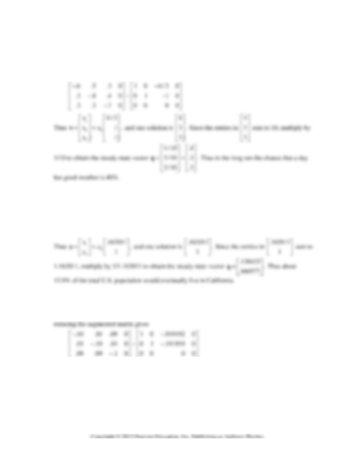
4. a. Let G stand for good weather, I for indifferent weather, and B for bad weather. Then the change
in the weather is given by the table
From:
G I B To:
.4 .5 .3 G
4.9 • Solutions 261
b. The initial state vector is
.5
.5 .
0
⎡⎤
⎢⎥
⎢⎥
⎢⎥
⎣⎦
We calculate
1
x
:
.4 .5 .3 .5 .45
⎡
⎤⎡ ⎤ ⎡ ⎤
c. The initial state vector is
0
0
.6 .
.4
⎡⎤
⎢⎥
=⎢⎥
⎢⎥
⎣⎦
x
We calculate
2
x
:
.4 .5 .3 0 .42
⎡
⎤⎡ ⎤ ⎡ ⎤
21
.4 .5 .3 .42 .398
.3 .2 .4 .28 .302
P
⎡
⎤⎡ ⎤ ⎡ ⎤
⎢
⎥⎢ ⎥ ⎢ ⎥
== =
xx
5. We solve Px = x by rewriting the equation as (P – I)x = 0, where
.9 .5 .
.9 .5
PI −
⎡
⎤
−=
⎢
⎥
−
⎣
⎦
Row reducing
the augmented matrix for the homogeneous system (P – I)x = 0 gives
.9 .5 0 1 5 / 9 0
−−
⎡⎤⎡⎤
6. We solve Px = x by rewriting the equation as (P – I)x = 0, where
.6 .8 .
.6 .8
PI −
⎡
⎤
−=
⎢
⎥
−
⎣
⎦
Row reducing
the augmented matrix for the homogeneous system (P – I)x = 0 gives
.6 .8 0 1 4 / 3 0
.6 .8 0 0 0 0
−−
⎡⎤⎡⎤
∼
⎢⎥⎢⎥
−
⎣⎦⎣⎦
262 CHAPTER 4 • Vector Spaces
7. We solve Px = x by rewriting the equation as (P – I)x = 0, where
.3 .1 .1
.2 .2 .2 .
.1 .1 .3
PI
−
⎡
⎤
⎢
⎥
−= −
⎢
⎥
⎢
⎥
−
⎣
⎦
Row
reducing the augmented matrix for the homogeneous system (P – I)x = 0 gives
.3 .1 .1 0 1 0 1 0
−−
⎡⎤⎡⎤
8. We solve Px = x by rewriting the equation as (P – I)x = 0, where
.6 .5 .8
0.5.1.
.6 0 .9
PI
−
⎡
⎤
⎢
⎥
−= −
⎢
⎥
⎢
⎥
−
⎣
⎦
Row
reducing the augmented matrix for the homogeneous system (P – I)x = 0 gives
.6 .5 .8 0 1 0 3 / 2 0
0.5.10 011/50
.6 0 .90 00 00
−−
⎡⎤⎡⎤
⎢⎥⎢⎥
−∼−
⎢⎥⎢⎥
⎢⎥⎢⎥
−
⎣⎦⎣⎦
9. Since
2.84 .2
.16 .8
P⎡⎤
=⎢⎥
⎣⎦
has all positive entries, P is a regular stochastic matrix.
10. Since
11.7
k
k
P
⎡⎤
−
=⎢⎥
will have a zero as its (2,1) entry for all k, P is not a regular stochastic
11. a. From Exercise 1,
.7 .6 ,
.3 .4
P⎡⎤
=⎢⎥
⎣⎦
so
.3 .6 .
.3 .6
PI −
⎡
⎤
−=
⎢
⎥
−
⎣
⎦
Solving (P – I)x = 0 by row reducing the
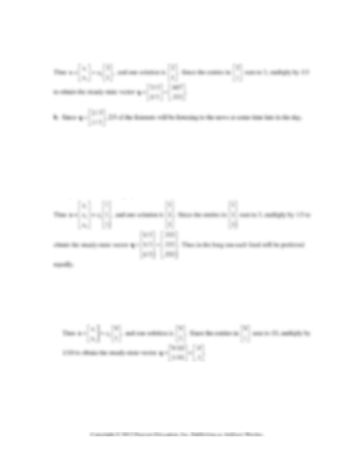
4.9 • Solutions 263
.3 .6 0 1 2 0
.3 .6 0 0 0 0
−−
⎡⎤⎡⎤
∼
⎢⎥⎢⎥
−
⎣⎦⎣⎦
12. From Exercise 2,
.6 .2 .2
.2 .6 .2 ,
.2 .2 .6
P
⎡
⎤
⎢
⎥
=
⎢
⎥
⎢
⎥
⎣
⎦
so
.4 .2 .2
.2 .4 .2 .
.2 .2 .4
PI
−
⎡
⎤
⎢
⎥
−= −
⎢
⎥
⎢
⎥
−
⎣
⎦
Solving (P – I)x = 0 by row
reducing the augmented matrix gives
.4 .2 .2 0 1 0 1 0
.2 .4 .2 0 0 1 1 0
.2 .2 .4 0 0 0 0 0
−−
⎡⎤⎡⎤
⎢⎥⎢⎥
−∼−
⎢⎥⎢⎥
⎢⎥⎢⎥
−
⎣⎦⎣⎦
13. a. From Exercise 3,
.95 .45 ,
.05 .55
P⎡⎤
=⎢⎥
⎣⎦
so
.05 .45 .
.05 .45
PI −
⎡
⎤
−=
⎢
⎥
−
⎣
⎦
Solving (P – I)x = 0 by row
reducing the augmented matrix gives
.05 .45 0 1 9 0
.05 .45 0 0 0 0
−−
⎡⎤⎡⎤
∼
⎢⎥⎢⎥
−
⎣⎦⎣⎦
b. After many days, a specific student is ill with probability .1, and it does not matter whether that
student is ill today or not.
264 CHAPTER 4 • Vector Spaces
14. From Exercise 4,
.4 .5 .3
.3 .2 .4 ,
.3 .3 .3
P
⎡
⎤
⎢
⎥
=
⎢
⎥
⎢
⎥
⎣
⎦
so
.6 .5 .3
.3 .8 .4 .
.3 .3 .7
PI
−
⎡
⎤
⎢
⎥
−= −
⎢
⎥
⎢
⎥
−
⎣
⎦
Solving (P – I)x = 0 by row
reducing the augmented matrix gives
15. [M] Let
.9821 .0029 ,
.0179 .9971
P⎡⎤
=⎢⎥
⎣⎦
so
.0179 .0029 .
.0179 .0029
PI −
⎡
⎤
−=
⎢
⎥
−
⎣
⎦
Solving (P – I)x = 0 by row reducing
the augmented matrix gives
.0179 .0029 0 1 .162011 0
.0179 .0029 0 0 0 0
−−
⎡⎤⎡⎤
∼
⎢⎥⎢⎥
−
⎣⎦⎣⎦
16. [M] Let
.90 .01 .09
.01 .90 .01 ,
.09 .09 .90
P
⎡⎤
⎢⎥
=⎢⎥
⎢⎥
⎣⎦
so
.10 .01 .09
.01 .10 .01 .
.09 .09 .1
PI
−
⎡
⎤
⎢
⎥
−= −
⎢
⎥
⎢
⎥
−
⎣
⎦
Solving (P – I)x = 0 by row
4.9 • Solutions 265
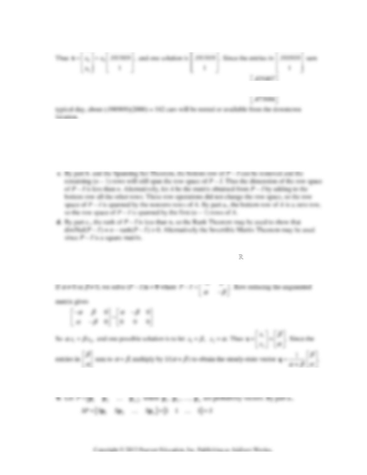
1
.919192
x
⎡⎤ ⎡ ⎤
.919192
⎡
⎤
.919192
⎡⎤
to 2.111111, multiply by 1/2.111111 to obtain the steady-state vector
.090909 .
⎡
⎤
⎢
⎥
=
⎢
⎥
q
Thus on a
17. a. The entries in each column of P sum to 1. Each column in the matrix P – I has the same entries as
in P except one of the entries is decreased by 1. Thus the entries in each column of P – I sum to 0,
and adding all of the other rows of P – I to its bottom row produces a row of zeros.
b . By part a., the bottom row of P – I is the negative of the sum of the other rows, so the rows of
P – I are linearly dependent.
18. If
α
=
β
= 0 then
10
.
01
P
⎡
⎤
=
⎢
⎥
⎣
⎦
Notice that Px = x for any vector x in
2
, and that
1
0
⎡⎤
⎢⎥
⎣⎦
and
0
1
⎡⎤
⎢⎥
⎣⎦
are
two linearly independent steady-state vectors in this case.
⎣
⎦
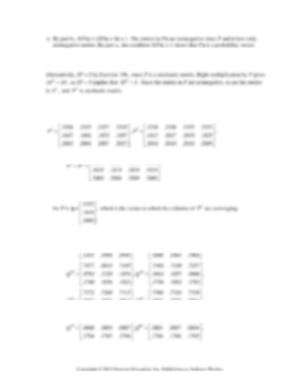
19. a. The product Sx equals the sum of the entries in x. Thus x is a probability vector if and only if its
entries are nonnegative and Sx = 1.
266 CHAPTER 4 • Vector Spaces
20. Let
[]
12
,
n
P=…pp p
so
[]
2
12 .
n
PPPP P P== …
pp p
By Exercise 19c., the columns
of
2
P
are probability vectors, so
2
P
is a stochastic matrix.
21. [M]
a. To four decimal places,
.2779 .2780 .2803 .2941 .2817 .2817 .2817 .2814
⎡⎤⎡⎤
.2816 .2816 .2816 .2816
.3355 .3355 .3355 .3355
⎡⎤
⎢⎥
The columns of
k
P
are converging to a common vector as k increases. The steady state vector q
.2816
⎡⎤
b. To four decimal places,
10 20
.8222 .4044 .5385 .7674 .6000 .6690
.0324 .3966 .1666 , .0637 .2036 .1326 ,
QQ
⎡⎤⎡⎤
⎢⎥⎢⎥
==
⎢⎥⎢⎥
.0867 .0951 .0913 , .0876 .0909 .0894 ,
.1761 .1780 .1772 .1763 .1771 .1767
QQ
==
⎢⎥⎢⎥
⎢⎥⎢⎥
⎣⎦⎣⎦
.7356 .7340 .7347 .7354 .7348 .7351
⎡⎤⎡⎤
Chapter 4 • Supplementary Exercises 267
.7353 .7353 .7353
⎡
⎤
c. Let P be an n × n regular stochastic matrix, q the steady state vector of P, and
j
e
the
th
j
column
[]
22. [M] Answers will vary.
MATLAB Student Version 4.0 code for Method (1):
A=randstoc(32); flops(0);
Chapter 4 SUPPLEMENTARY EXERCISES
1. a. True. This set is
1
Span{ ,... }
p
vv
, and every subspace is itself a vector space.
b. True. Any linear combination of
1
v
, …,
1p−
v
is also a linear combination of
1
v
, …,
1p−
v
,
p
v
using the zero weight on
.
p
v
g. False. The plane must pass through the origin to be a subspace.
h. False. Counterexample:
25 20
00 73
−
⎡⎤
⎢⎥
⎢⎥
.
m. True. Row equivalent matrices have the same number of pivot columns.
n. False. The nonzero rows of A span Row A but they may not be linearly independent.
o. True. The nonzero rows of the reduced echelon form E form a basis for the row space of each
matrix that is row equivalent to E.
p. True. If H is the zero subspace, let A be the 3 × 3 zero matrix. If dim H = 1, let {v} be a basis
s. True. See the second paragraph after Theorem 15 in Section 4.7.
t. False. The
th
j
column of
CB
P
←
is
.
jC
⎡
⎤
⎣
⎦
b
2. The set is SpanS, where
125
258
,, .
147
311
S
⎧⎫−
⎡⎤⎡⎤⎡⎤
⎪⎪
⎢⎥⎢⎥⎢⎥
−
⎪⎪
⎢⎥⎢⎥⎢⎥
=⎨⎬
⎢⎥⎢⎥⎢⎥
−−
⎪⎪
⎢⎥⎢⎥⎢⎥
⎪⎪
⎢⎥⎢⎥⎢⎥
⎣⎦⎣⎦⎣⎦
⎩⎭
Note that S is a linearly dependent set, but each
3. The vector b will be in
12
Span{ , }W=
uu
if and only if there exist constants
1
c
and
2
c
with
11 2 2
.cc+=
uub
Row reducing the augmented matrix gives
4. The vector g is not a scalar multiple of the vector f, and f is not a scalar multiple of g, so the set
{f, g} is linearly independent. Even though the number g(t) is a scalar multiple of f(t) for each t, the
scalar depends on t.
6. Find two polynomials from the set
14
{,..., }
pp
that are not multiples of one another. This is easy,
7. You would have to know that the solution set of the homogeneous system is spanned by two
solutions. In this case, the null space of the 18 × 20 coefficient matrix A is at most two-dimensional.
8. If n = 0, then H and V are both the zero subspace, and H = V. If n > 0, then a basis for H consists of n
9. Let T:
n
⎯
→
m
be a linear transformation, and let A be the m × n standard matrix of T.
a. If T is one-to-one, then the columns of A are linearly independent by Theorem 12 in Section 1.9,
so dimNul A = 0. By the Rank Theorem, dimCol A = n – 0 = n, which is the number of columns
of A. As noted in Section 4.2, the range of T is Col A, so the dimension of the range of T is n.
10. Let
1
{,..., }.
p
S=vv
If S were linearly independent and not a basis for V, then S would not span V.
11. If S is a finite spanning set for V, then a subset of S is a basis for V. Denote this subset of S by .S′
12. a. Let y be in Col AB. Then y = ABx for some x. But ABx = A(Bx), so y = A(Bx), and y is in Col A.
Thus Col AB is a subspace of Col A, so rank AB = dimCol AB ≤ dimCol A = rank A by Theorem
11 in Section 4.5.
13. By Exercise 12, rank PA ≤ rank A, and
11
rank rank( ) rank ( ) rankAPPAPPAPA
−−
== ≤
, so
14. Note that
() .
TTT
AQ Q A=
Since
T
Q
is invertible, we can use Exercise 13 to conclude that
15. The equation AB = O shows that each column of B is in Nul A. Since Nul A is a subspace of
n
, all
linear combinations of the columns of B are in Nul A. That is, Col B is a subspace of Nul A. By
16. Suppose that
1
rank Ar=
and
2
rank Br=
. Then there are rank factorizations
11
ACR=
and
22
BCR=
of A and B, where
1
C
is
1
mr×
with rank
1
r
,
2
C
is
2
mr×
with rank
2
r
,
1
R
is
1
rn×
with rank
1
r
, and
2
R
is
2
rn×
with rank
2
.r
Create an
12
()mrr×+
matrix
[]
12
CCC=
and an
12
()rr n+×
matrix R
by stacking
1
R
over
2
.
R
Then
17. Let A be an m × n matrix with rank r.
(a) Let
1
A
consist of the r pivot columns of A. The columns of
1
A
are linearly independent, so
1
A
18. Let A be a 4 × 4 matrix and B be a 4 × 2 matrix, and let
03
,...,
uu
be a sequence of input vectors in
2
.
a. Use the equation
1kkk
AB
+
=+
xxu
for
0,..., 4,k=
with
0
.=
x0

Chapter 4 • Supplementary Exercises 271
2
322 01 2 0 12
()AB AABB B ABABB=+= + += + +xxu uu u u uu
b. If (A, B) is controllable, then the controllability matrix has rank 4, with a pivot in each row, and
the columns of M span
4
. Therefore, for any vector v in
4
, there is a vector u in
8
such that
19. To determine if the matrix pair (A, B) is controllable, we compute the rank of the matrix
2
.BABAB
⎡⎤
⎣⎦
To find the rank, we row reduce:
20. To determine if the matrix pair (A, B) is controllable, we compute the rank of the matrix
2
.BABAB
⎡⎤
⎣⎦
To find the rank, we note that :
1.5.19
⎡⎤
21. [M] To determine if the matrix pair (A, B) is controllable, we compute the rank of the matrix
23
.BABABAB
⎡⎤
⎣⎦
To find the rank, we row reduce:
10 0 1 100 1
−−
⎡⎤⎡⎤
22. [M] To determine if the matrix pair (A, B) is controllable, we compute the rank of the matrix
23
.BABABAB
⎡⎤
⎣⎦
To find the rank, we row reduce: