2.5 • Solutions 127
1
Likewise to find ,U
−
[]
row reduce :UI
[]
242100 240102 2401 02
036010~030016~01001/32
001001 001001 0010 01
UI
−−−−−
⎡⎤⎡ ⎤⎡ ⎤
⎢⎥⎢ ⎥⎢ ⎥
=− − − −
⎢⎥⎢ ⎥⎢ ⎥
⎢⎥⎢ ⎥⎢ ⎥
⎣⎦⎣ ⎦⎣ ⎦
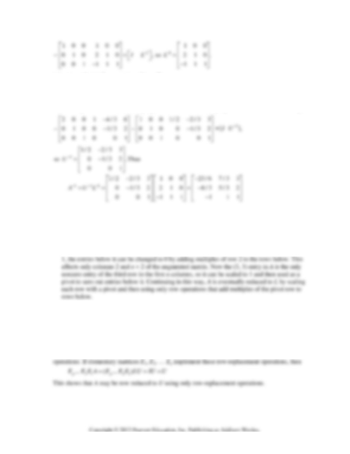
19. Let A be a lower-triangular n × n matrix with nonzero entries on the diagonal, and consider the
augmented matrix [A I].
a. The (1, 1)-entry can be scaled to 1 and the entries below it can be changed to 0 by adding
multiples of row 1 to the rows below. This affects only the first column of A and the first column
of I. So the (2, 2)-entry in the new matrix is still nonzero and now is the only nonzero entry of
row 2 in the first n columns (because A was lower triangular). The (2, 2)-entry can be scaled to
b. The row operations just described only add rows to rows below, so the I on the right in [A I]
changes into a lower triangular matrix. By Theorem 7 in Section 2.2, that matrix is A
–1
.
20. Let A
= LU be an LU factorization for A. Since L is unit lower triangular, it is invertible by Exercise
19. Thus by the Invertible Matrix Theroem, L may be row reduced to I. But L is unit lower triangular,
so it can be row reduced to I by adding suitable multiples of a row to the rows below it, beginning
with the top row. Note that all of the described row operations done to L are row-replacement
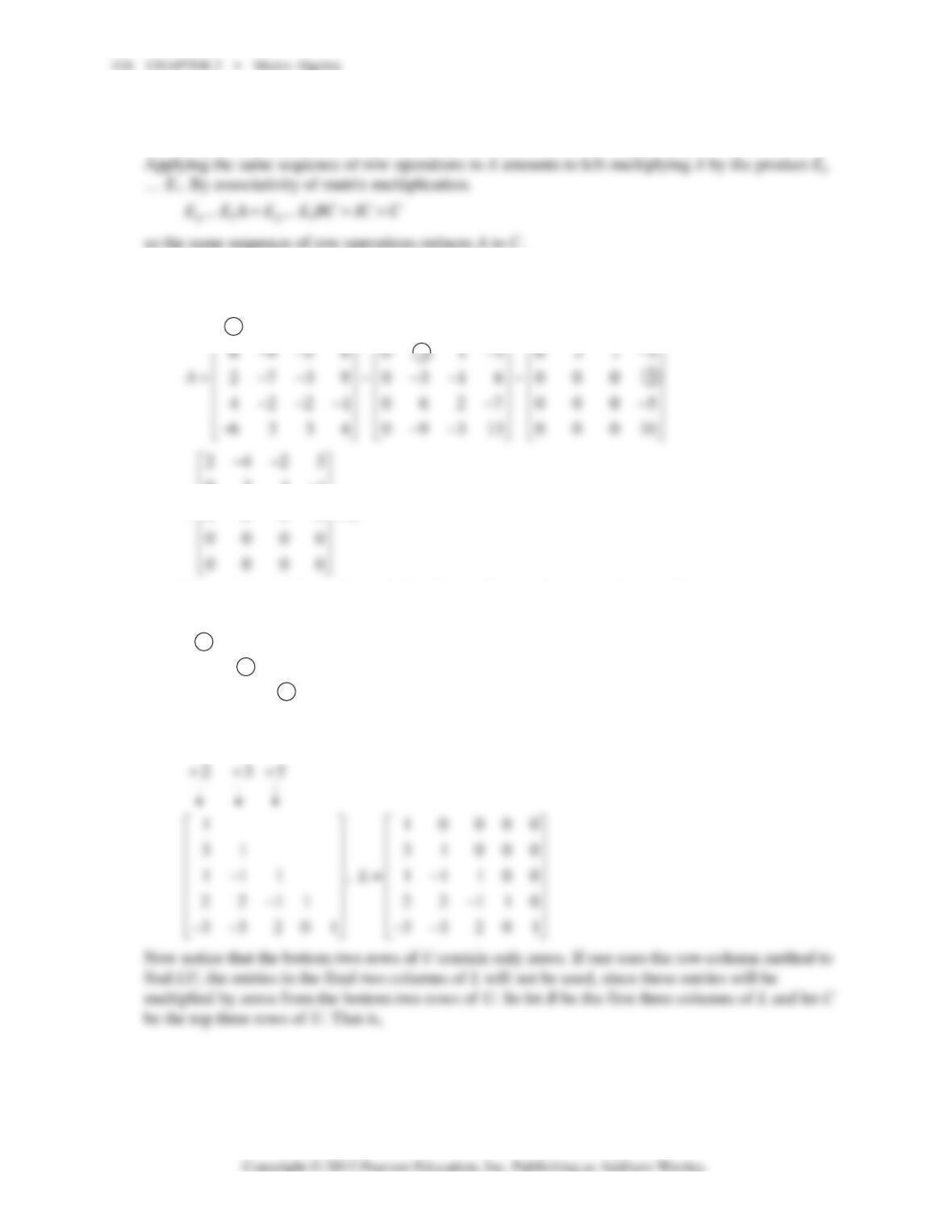
21. (Solution in Study Guide.) Suppose A = BC, with B invertible. Then there exist elementary matrices
E
1
, …, E
p
corresponding to row operations that reduce B to I, in the sense that E
p
… E
1
B = I.
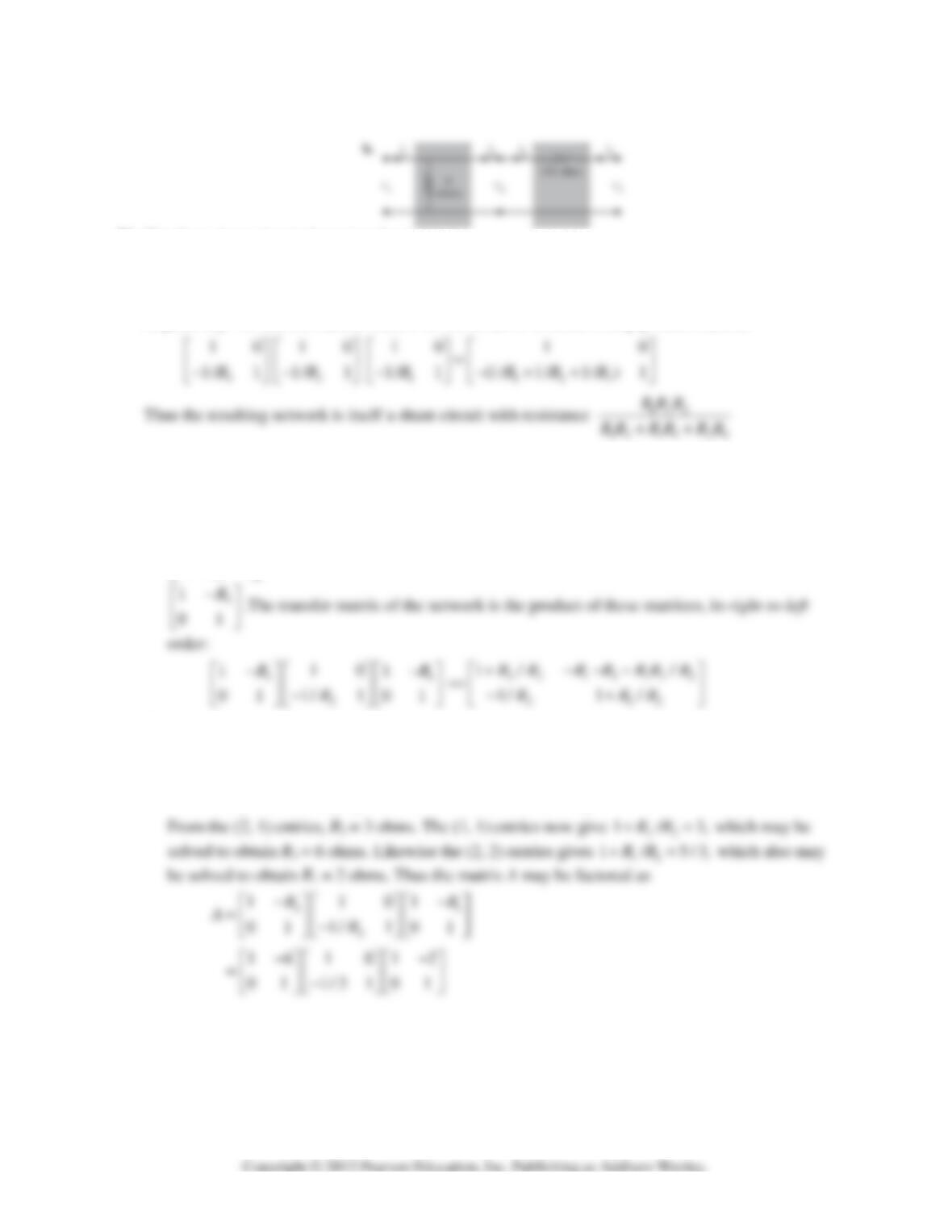
22. First find an LU factorization for A. Row reduce A to echelon form using only row replacement
operations:
2423 2423 2423
−− −− −−
⎡⎤⎡⎤⎡⎤
⎢⎥⎢⎥⎢⎥
0311
~0005
U
−
⎢⎥
⎢⎥
=
then follow the algorithm in Example 2 to find L. Use the last two columns of I
5
to make L unit lower
triangular.
2
63
5
23
5
46
10
69
⎡⎤
⎢⎥
⎡⎤
⎢⎥
⎢⎥
⎢⎥−⎡⎤
⎢⎥
⎢⎥ ⎢⎥
⎢⎥
−
⎢⎥ ⎢⎥
⎢⎥
⎢⎥ ⎢⎥
−−
⎣⎦
⎣⎦⎣⎦
2.5 • Solutions 129
100
⎡⎤
⎢⎥
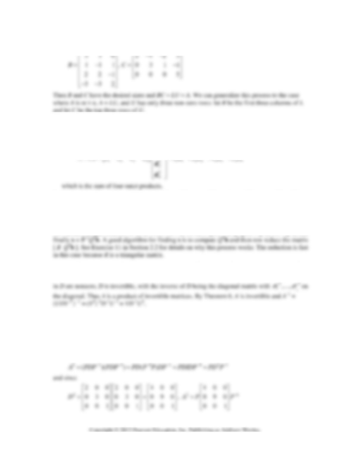
23. a. Express each row of D as the transpose of a column vector. Then use the multiplication rule for
partitioned matrices to write
1
2
T
T
T
TTT
ACD
⎡⎤
⎢⎥
⎢⎥
== = + + +
d
d
c c c c cd cd cd cd
b. Since A has 400 × 100 = 40000 entries, C has 400 × 4 = 1600 entries and D has 4 × 100 = 400
entries, to store C and D together requires only 2000 entries, which is 5% of the amount of entries
needed to store A directly.
24. Since Q is square and Q
T
Q = I, Q is invertible by the Invertible Matrix Theorem and Q
–1
= Q
T
. Thus
A is the product of invertible matrices and hence is invertible. Thus by Theorem 5, the equation
Ax = b has a unique solution for all b. From Ax = b, we have QRx = b, Q
T
QRx = Q
T
b, Rx = Q
T
b, and
25. A = UDV
T
. Since U and V
T
are square, the equations U
T
U = I and V
T
V = I imply that U and V
T
are invertible, by the IMT, and hence U
–1
= U
T
and (V
T
)
–1
= V. Since the diagonal entries
1,,
n
σσ
…
26. If A = PDP
–1
, where P is an invertible 3 × 3 matrix and D is the diagonal matrix
200
030
001
D
⎡⎤
⎢⎥
=⎢⎥
⎢⎥
⎣⎦
then
130 CHAPTER 2 • Matrix Algebra
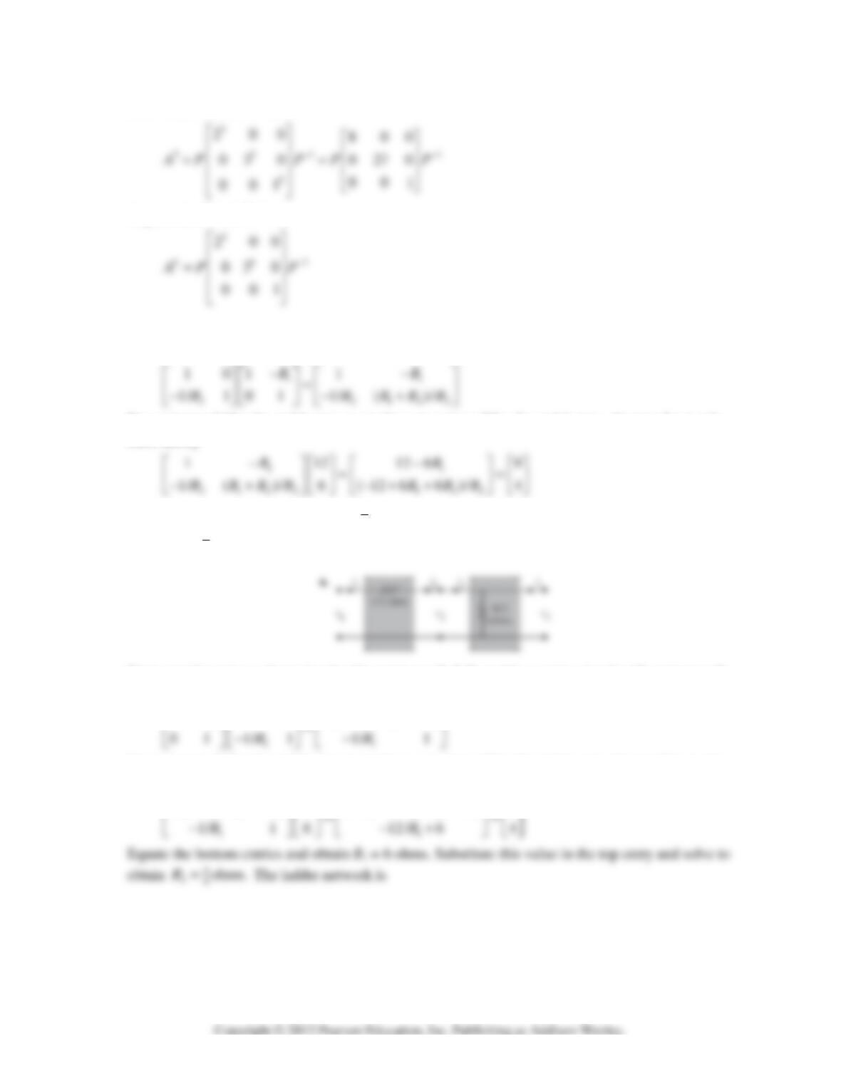
Likewise, A
3
= PD
3
P
–1
, so
In general, A
k
= PD
k
P
–1
, so
27. First consider using a series circuit with resistance R
1
followed by a shunt circuit with resistance R
2
for the network. The transfer matrix for this network is
R
For an input of 12 volts and 6 amps to produce an output of 9 volts and 4 amps, the transfer matrix
must satisfy
Equate the top entries and obtain
1
12
ohm.R=
Substitute this value in the bottom entry and solve to
obtain
9
22
ohms.R=
The ladder network is
Next consider using a shunt circuit with resistance R
1
followed by a series circuit with resistance R
2
for the network. The transfer matrix for this network is
121 2
2
10( )/1
R
RR RR
+−−⎡⎤⎡ ⎤
⎡⎤ =
For an input of 12 volts and 6 amps to produce an output of 9 volts and 4 amps, the transfer matrix
must satisfy
121 2 1 21 2
( ) / (12 12 ) / 612 9
RRR R R RR R
+− +−
⎡⎤⎡ ⎤
⎡⎤ ⎡⎤
2.5 • Solutions 131
28. The three shunt circuits have transfer matrices
312
10
10 10
,,and
1/ 1
1/ 1 1/ 1 R
RR
⎡⎤⎡⎤⎡⎤
⎢⎥
⎢⎥⎢⎥
−
−−
⎣⎦⎣⎦
⎣⎦
respectively. To find the transfer matrix for the series of circuits, multiply these matrices
29. a. The first circuit is a series circuit with resistance R
1
ohms, so its transfer matrix is
1
1
01
R
−
⎡⎤
⎢⎥
⎣⎦
.
The second circuit is a shunt circuit with resistance R
2
ohms, so its transfer matrix is
2
10
.
1/ 1R
⎡⎤
⎢⎥
−
⎣⎦
The third circuit is a series circuit with resistance R
3
ohms so its transfer matrix is
R
R
b. To find a ladder network with a structure like that in part (a) and with the given transfer matrix A,
we must find resistances R
1
, R
2
, and R
3
such that
32 13 132
212
1/ /
312
1/ 1 /
1/3 5/3
R
RRRRRR
ARRR
+−−−
−⎡⎤
⎡⎤
==
⎢⎥
⎢⎥
−+
−
⎣⎦
⎣⎦
R
30. Answers may vary. For example,
3 12161 01 012
1/3 5/3 0 1 1/6 1 1/6 1 0 1
−− −
⎡ ⎤⎡⎤⎡⎤⎡⎤⎡⎤
=
⎢ ⎥⎢⎥⎢⎥⎢⎥⎢⎥
−−−
⎣ ⎦⎣⎦⎣⎦⎣⎦⎣⎦
132 CHAPTER 2 • Matrix Algebra
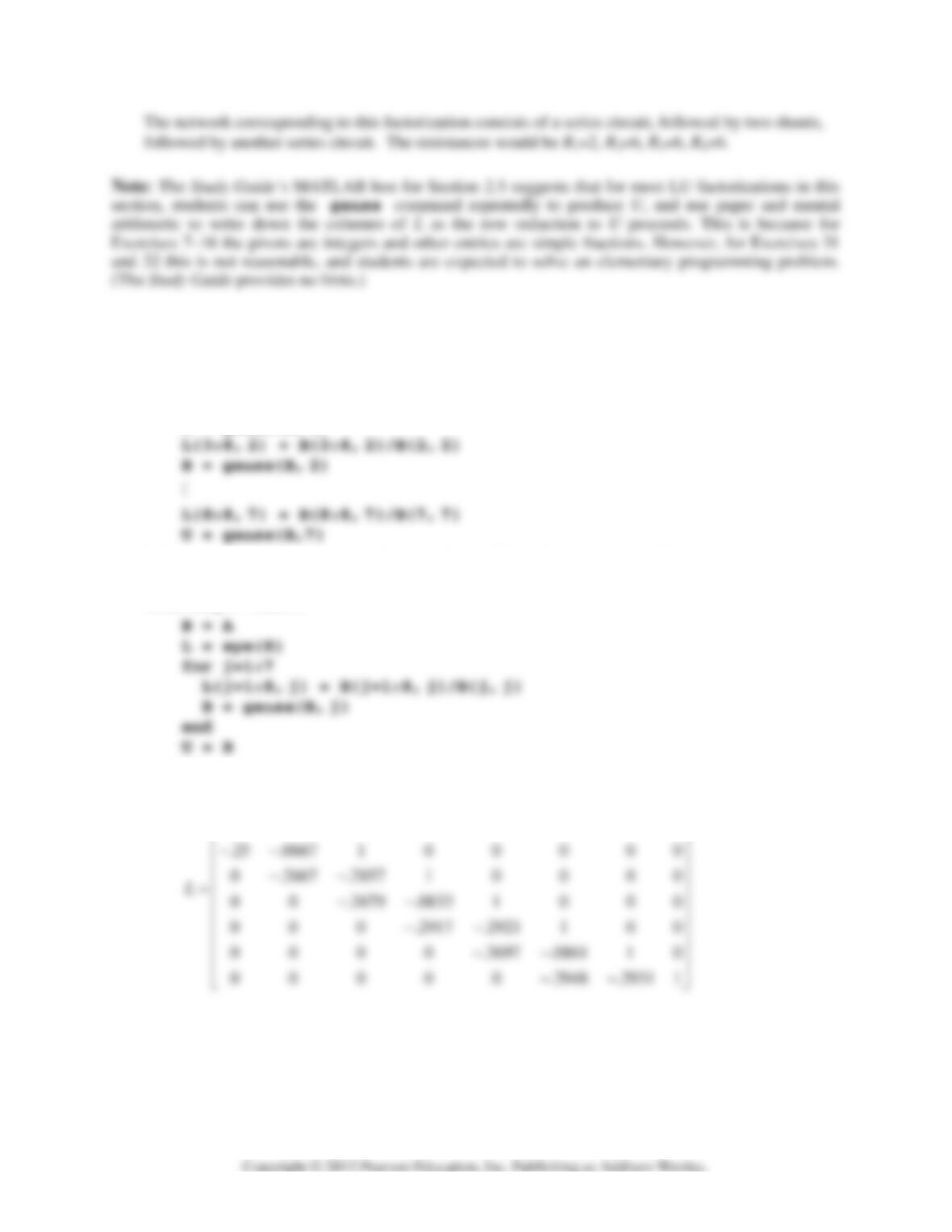
31. [M] Store the matrix A in a temporary matrix B and create L initially as the 8×8 identity matrix. The
following sequence of MATLAB commands fills in the entries of L below the diagonal, one column
at a time, until the first seven columns are filled. (The eighth column is the final column of the
identity matrix.)
L(2:8, 1) = B(2:8, 1)/B(1, 1)
B = gauss(B, 1)
Of course, some students may realize that a loop will speed up the process. The for..end syntax
is illustrated in the MATLAB box for Section 5.6. Here is a MATLAB program that includes the
initial setup of B and L:
a. To four decimal places, the results of the LU decomposition are
10000000
.251000000
⎡⎤
⎢⎥
−
⎢⎥
2.5 • Solutions 133
41 1 0 0 0 0 0
03.75 .25 1 0 0 0 0
−−
⎡⎤
⎢⎥
−−
⎢⎥
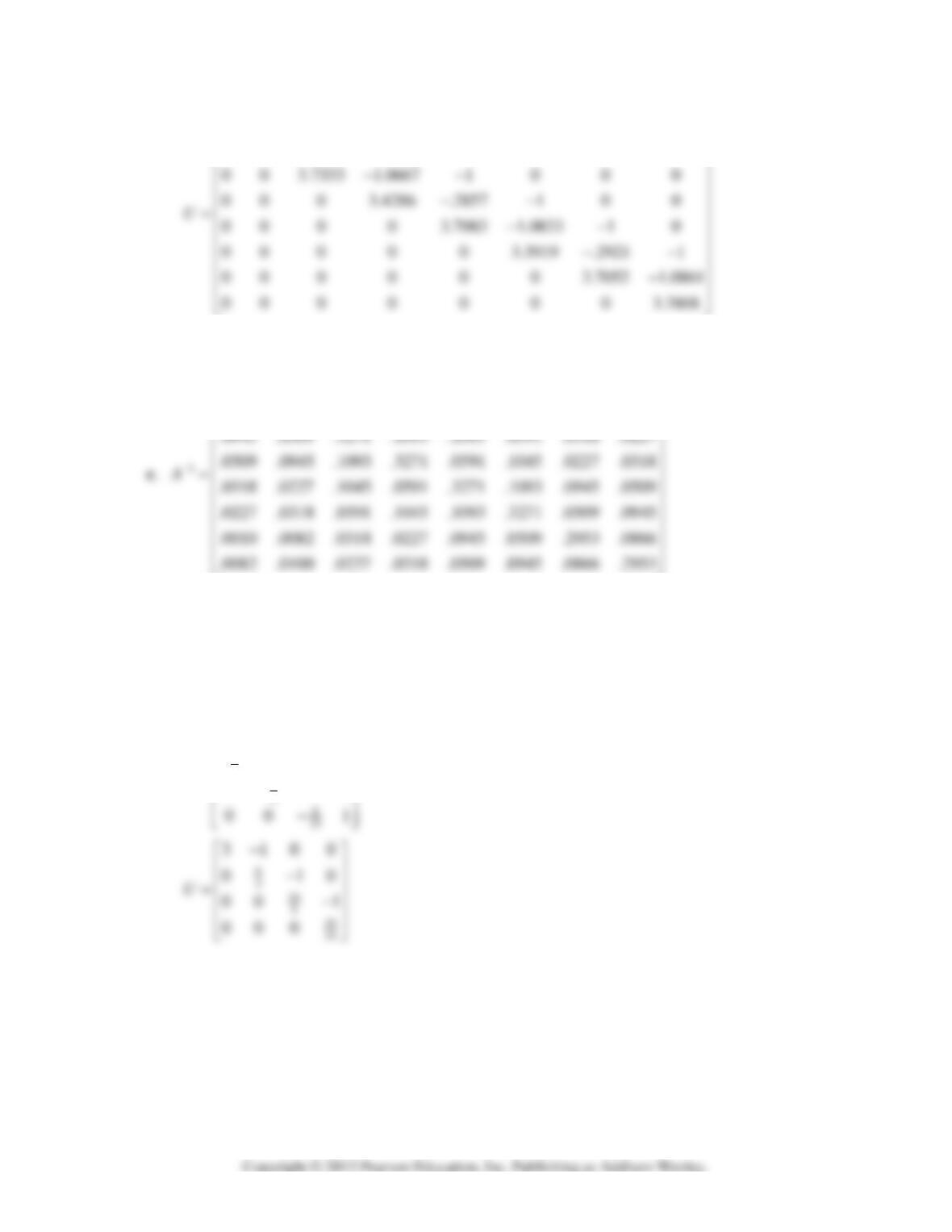
b. The result of solving Ly = b and then Ux = y is
x = (27.1292, 19.2344, 29.2823, 19.8086, 30.1914, 20.7177, 30.7656, 22.8708)
.2953 .0866 .0945 .0509 .0318 .0227 .0010 .0082
.0866 .2953 .0509 .0945 .0227 .0318 .0082 .0100
⎡⎤
⎢⎥
⎢⎥
⎣⎦
32. [M]
3100
1310
0131
0013
A
−
⎡⎤
⎢⎥
−−
⎢⎥
=⎢⎥
−−
⎢⎥
−
⎣⎦
. The commands shown for Exercise 31, but modified for 4×4 matrices,
produce
1
3
3
8
10 00
100
010
L
⎡⎤
⎢⎥
−
⎢⎥
=⎢⎥
−
2.4 • Solutions 134
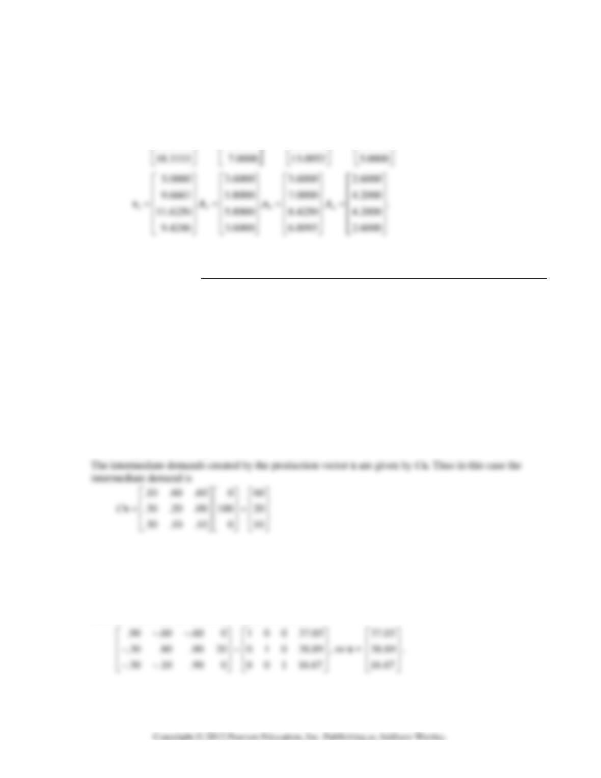
b. Let s
k+1
be the solution of Ls
k+1
= t
k
for k = 0, 1, 2, …. Then t
k+1
is the solution of Ut
k+1
= s
k+1
for k = 0, 1, 2, …. The results are
1122
10.0000 7.0000 7.0000 5.0000
18.3333 11.0000 13.3333 8.0000
,, ,,
21.8750 11.0000 16.0000 8.0000
⎡⎤⎡⎤⎡⎤⎡⎤
⎢⎥⎢⎥⎢⎥⎢⎥
⎢⎥⎢⎥⎢⎥⎢⎥
====
⎢⎥⎢⎥⎢⎥⎢⎥
stst
2.6 SOLUTIONS
Notes:
This section is independent of Section 1.10. The material here makes a good backdrop for the
series expansion of (I–C)
–1
because this formula is actually used in some practical economic work.
Exercise 8 gives an interpretation to entries of an inverse matrix that could be stated without the economic
context.
1. The answer to this exercise will depend upon the order in which the student chooses to list the
sectors. The important fact to remember is that each column is the unit consumption vector for the
appropriate sector. If we order the sectors manufacturing, agriculture, and services, then the
consumption matrix is
.10 .60 .60
.30 .20 0
.30 .10 .10
C
⎡⎤
⎢⎥
=⎢⎥
⎢⎥
⎣⎦
2. Solve the equation x = Cx + d for d:
11123
2212
33123
.10 .60 .60 .9 .6 .6 0
.30 .20 .00 .3 .8 20
.30 .10 .10 .3 .1 .9 0
xxxxx
Cx x x x
xxxxx
−−
⎡⎤ ⎡⎤⎡ ⎤⎡⎤ ⎡⎤
⎢⎥ ⎢⎥⎢ ⎥⎢⎥ ⎢⎥
=− = − =− + =
⎢⎥ ⎢⎥⎢ ⎥⎢⎥ ⎢⎥
⎢⎥ ⎢⎥⎢ ⎥⎢⎥ ⎢⎥
−−+
⎣⎦ ⎣⎦⎣⎦ ⎣⎦⎣ ⎦
dx x
This system of equations has the augmented matrix
3. Solving as in Exercise 2:
11123
2212
33123
.10 .60 .60 .9 .6 .6 20
.30 .20 .00 .3 .8 0
.30 .10 .10 .3 .1 .9 0
xxxxx
xxxx
xxxxx
−−
⎡⎤ ⎡⎤⎡ ⎤⎡⎤ ⎡⎤
⎢⎥ ⎢⎥⎢ ⎥⎢⎥ ⎢⎥
=− = − =− + =
⎢⎥ ⎢⎥⎢ ⎥⎢⎥ ⎢⎥
⎢⎥ ⎢⎥⎢ ⎥⎢⎥ ⎢⎥
−−+
⎣⎦ ⎣⎦⎣⎦ ⎣⎦⎣ ⎦
dx xC
This system of equations has the augmented matrix
⎡
⎢
⎢
⎢
⎣
4. Solving as in Exercise 2:
11123
2212
33123
.10 .60 .60 .9 .6 .6 20
.30 .20 .00 .3 .8 20
.30 .10 .10 .3 .1 .9 0
xxxxx
Cx x x x
xxxxx
−−
⎡⎤ ⎡⎤⎡ ⎤⎡⎤ ⎡⎤
⎢⎥ ⎢⎥⎢ ⎥⎢⎥ ⎢⎥
=− = − =− + =
⎢⎥ ⎢⎥⎢ ⎥⎢⎥ ⎢⎥
⎢⎥ ⎢⎥⎢ ⎥⎢⎥ ⎢⎥
−−+
⎣⎦ ⎣⎦⎣⎦ ⎣⎦⎣ ⎦
dx x
This system of equations has the augmented matrix
⎢
⎢
⎢
⎣
.90 .60 .60 20 1 0 0 81.48
−−
⎡⎤⎡⎤
81.48
⎡
⎤
Note:
Exercises 2–4 may be used by students to discover the linearity of the Leontief model.
5.
1
1
1.5501.6150110
() .6 .8 30 1.2 2 30 120
IC
−
−
−
⎡ ⎤⎡⎤⎡ ⎤⎡⎤⎡ ⎤
=− = = =
⎢ ⎥⎢⎥⎢ ⎥⎢⎥⎢ ⎥
−
⎣ ⎦⎣⎦⎣ ⎦⎣⎦⎣ ⎦
xd
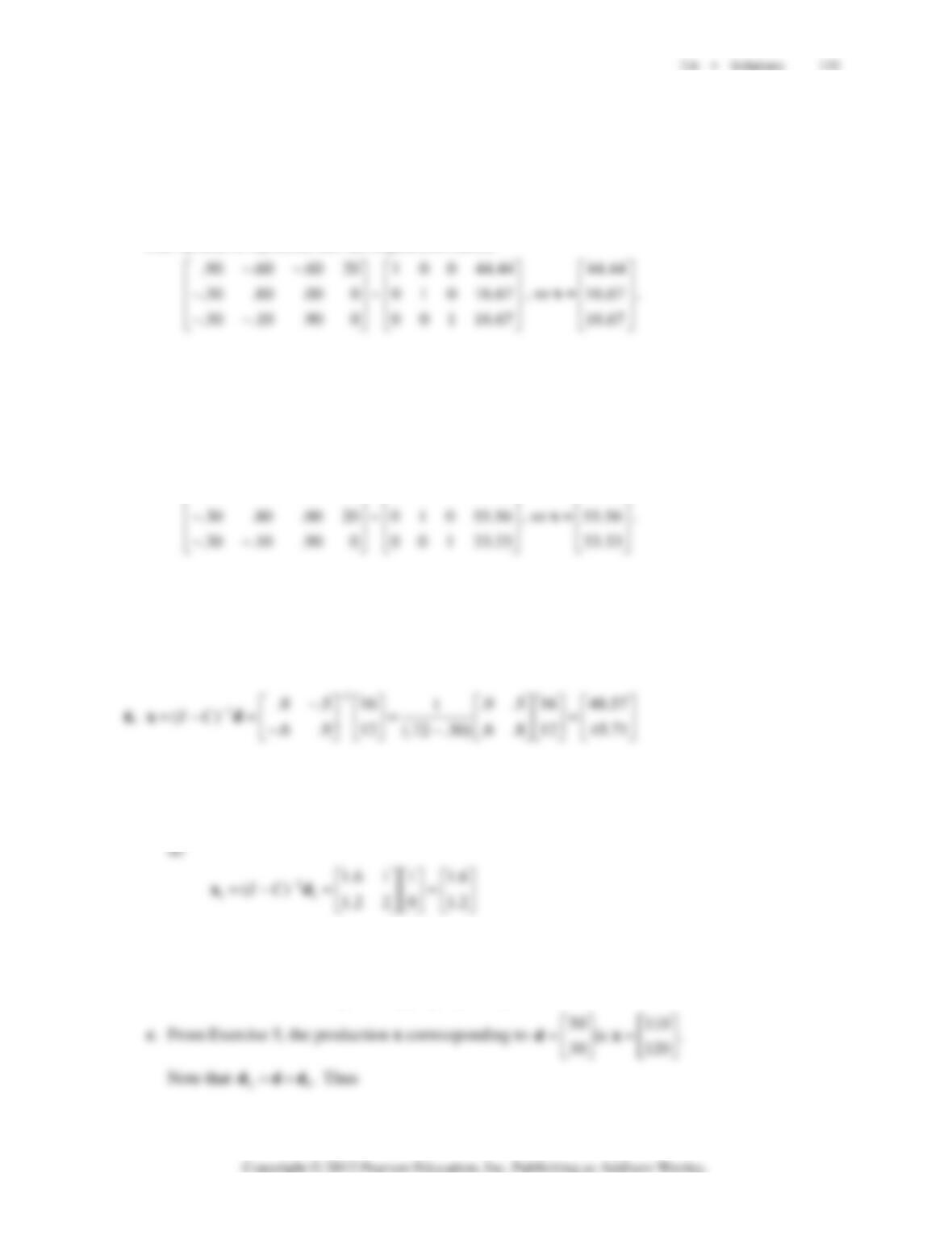
7. a. From Exercise 5,
11.6 1
()1.2 2
IC
−
⎡
⎤
−=
⎢
⎥
⎣
⎦
which is the first column of
1
().IC
−
−
b.
1
22
1.6 1 51 111.6
() 1.2 2 30 121.2
IC
−⎡⎤⎡⎤⎡⎤
=− = =
⎢⎥⎢⎥⎢⎥
⎣⎦⎣⎦⎣⎦
xd
⎡
⎢
⎣
136 CHAPTER 2 • Matrix Algebra
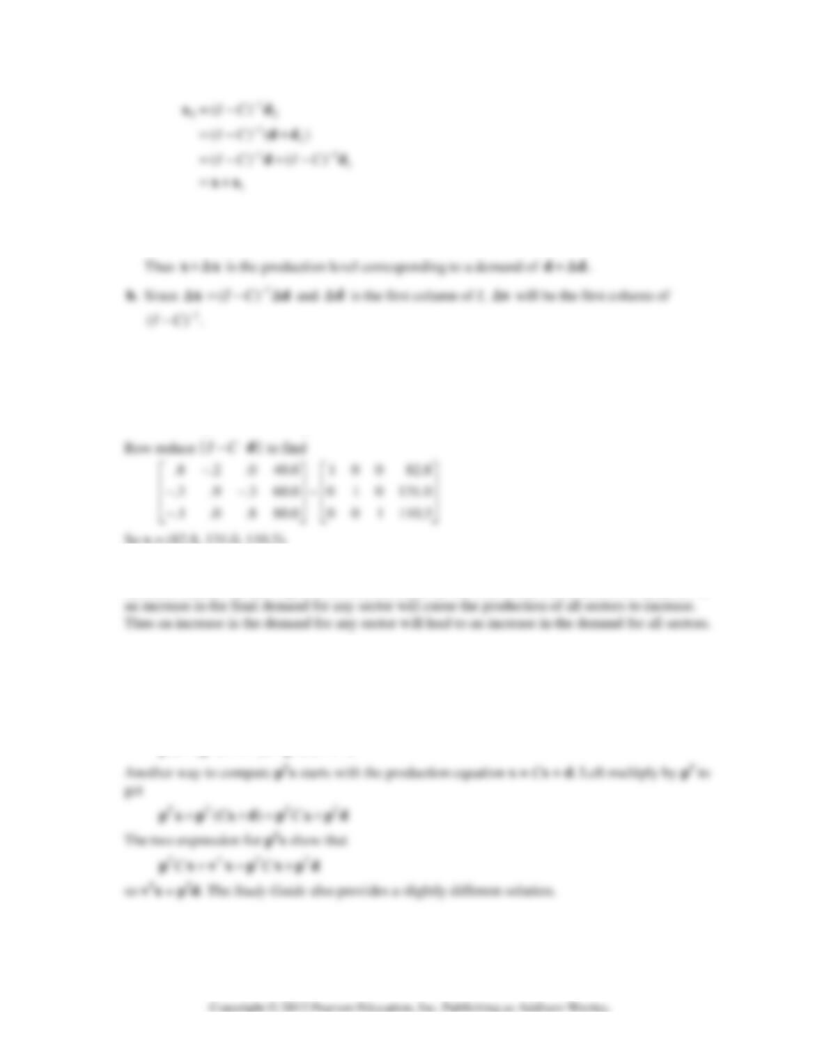
8. a. Given () and() ,IC IC−= − =xd x dΔΔ
()( )()()IC IC IC−+=−+− =+xx x xddΔΔΔ
9. In this case
.8 .2 .0
.3 .9 .3
.1 .0 .8
IC
−
⎡⎤
⎢⎥
−=− −
⎢⎥
⎢⎥
−
⎣⎦
So x = (82.8, 131.0, 110.3).
10. From Exercise 8, the (i, j) entry in (I – C)
–1
corresponds to the effect on production of sector i when
the final demand for the output of sector j increases by one unit. Since these entries are all positive,
11. (Solution in study Guide) Following the hint in the text, compute p
T
x in two ways. First, take the
transpose of both sides of the price equation, p = C
T
p + v, to obtain
(v)()
TT TTTTT T
CC C=+= +=+pp pvpv
and right-multiply by x to get
()
TTT T T
CC=+= +px p v x p x v x
2.6 • Solutions 137
12. Since
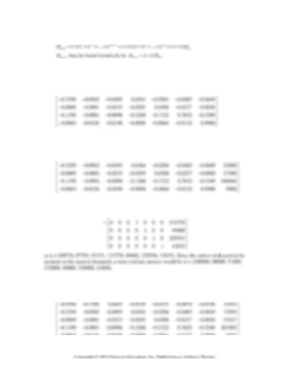
13. [M] The matrix I – C is
0.8412 0.0064 0.0025 0.0304 0.0014 0.0083 0.1594
0.0057 0.7355 0.0436 0.0099 0.0083 0.0201 0.3413
0.0264 0.1506 0.6443 0.0139 0.0142 0.0070 0.0236
−−−−−−
−−−−−−
−− −−−−
⎡⎤
⎢⎥
⎢⎥
⎢⎥
so the augmented matrix []IC−d may be row reduced to find
0.8412 0.0064 0.0025 0.0304 0.0014 0.0083 0.1594 74000
0.0057 0.7355 0.0436 0.0099 0.0083 0.0201 0.3413 56000
0.0264 0.1506 0.6443 0.0139 0.0142 0.0070 0.0236 10500
−−−−−−
−−−−−−
−− −−−−
⎡ ⎤
⎢ ⎥
⎢ ⎥
⎢ ⎥
1 0 0 0 0 0 0 99576
0 1 0 0 0 0 0 97703
0 0 1 0 0 0 0 51231
⎡⎤
⎢⎥
⎢⎥
⎢⎥
14. [M] The augmented matrix []IC−d in this case may be row reduced to find
0.8412 0.0064 0.0025 0.0304 0.0014 0.0083 0.1594 99640
0.0057 0.7355 0.0436 0.0099 0.0083 0.0201 0.3413 75548
−−−−−−
−−−−−−
0.0063 0.0126 0.0196 0.0098 0.0064 0.0132 0.9988 6526
⎡ ⎤
⎢ ⎥
⎢ ⎥
−−−−−−
⎣ ⎦

138 CHAPTER 2 • Matrix Algebra
1000000134034
0 0 0 0 0 0 1 18431
⎡⎤
⎢⎥
⎢⎥
⎣⎦
so x = (134034, 131687, 69472, 176912, 66596, 443773, 18431). To the nearest thousand, x =
15. [M] Here are the iterations rounded to the nearest tenth:
(0)
(2)
(74000.0, 56000.0, 10500.0, 25000.0, 17500.0, 196000.0, 5000.0)
(94681.2, 87714.5, 37577.3, 100520.5, 38598.0, 296563.8, 11480.0)
=
=
=
=
x
x
x
(4)
(6)
(98291.6, 95033.2, 47314.5, 123202.5, 46247.0, 320502.4, 13185.5)
(99226.6, 96969.
=
=
x
x
(8)
6, 50139.6, 129296.7, 48569.3, 327053.8, 13655.9)
(99480.0, 97500.7, 50928.7, 130948.0, 49232.5, 328864.7, 13785.9)
=
=
=
x
x
x
(10)
(99549.4, 97647.2, 51147.2, 131399.2, 49417.7, 329364.4, 13821.7)
=
=
x
x
so x
(12)
is the first vector whose entries are accurate to the nearest thousand. The calculation of x
(12)
takes about 1260 flops, while the row reduction above takes about 550 flops. If C is larger than
2.7 SOLUTIONS
Notes:
The content of this section seems to have universal appeal with students. It also provides practice
2.7 • Solutions 139
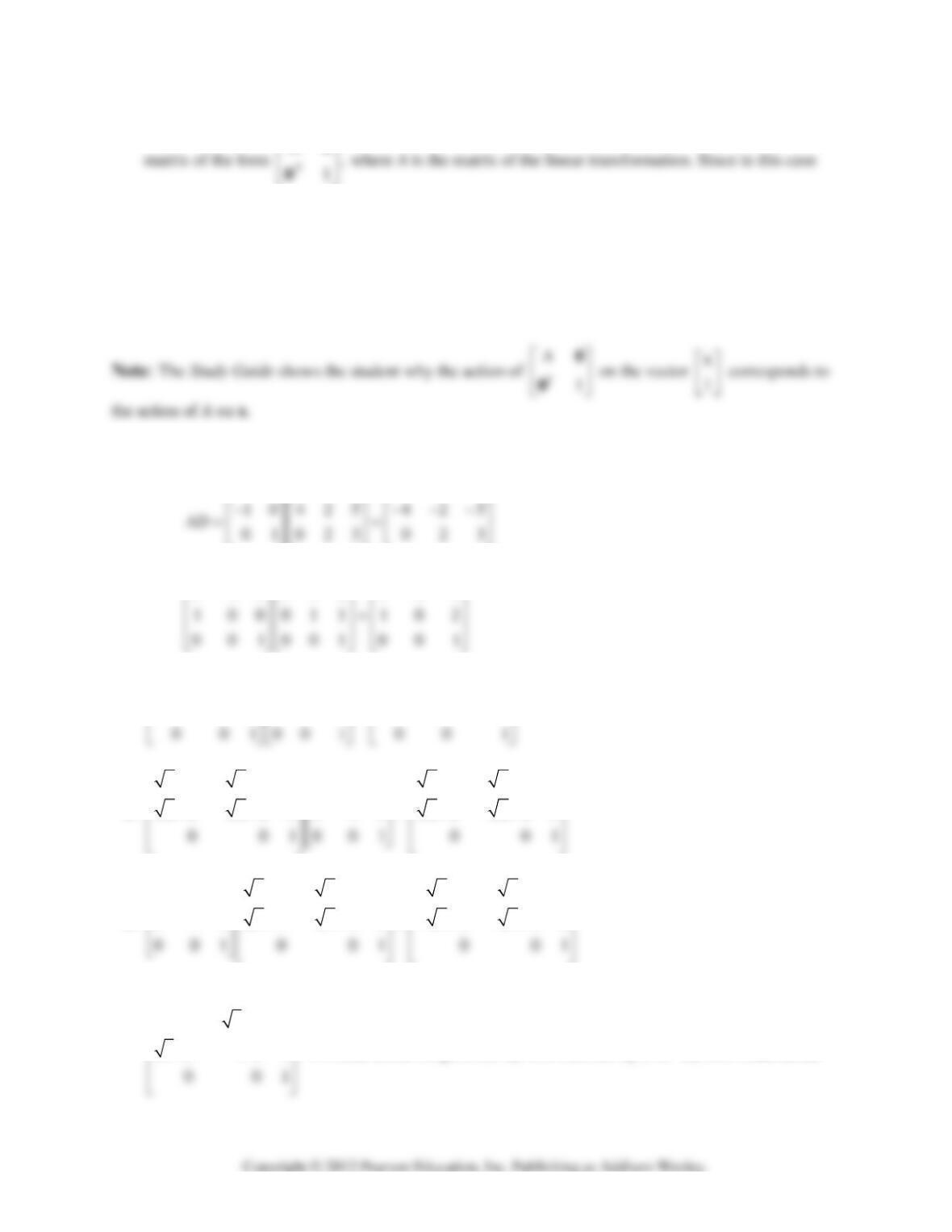
1. Refer to Example 5. The representation in homogenous coordinates can be written as a partitioned
A
⎡⎤
0
1.25
,
01
A⎡⎤
=⎢⎥
⎣⎦
the representation of the transformation with respect to homogenous coordinates is
1.25 0
010
001
⎡⎤
⎢⎥
⎢⎥
⎢⎥
⎣⎦
2. The matrix of the transformation is
10
01
A−
⎡
⎤
=
⎢
⎥
⎣
⎦
, so the transformed data matrix is
3. Following Examples 4–6,
010102 011
−−−
⎡⎤⎡⎤⎡ ⎤
4.
1/ 2 0 0 1 0 1 1/ 2 0 1/ 2
03/2001 4 03/2 6
−−
⎡⎤⎡⎤⎡ ⎤
⎢⎥⎢⎥⎢ ⎥
=
⎢⎥⎢⎥⎢ ⎥
5.
2/2 2/2 0 2/2 2/2 0
100
2/22/20010 2/22/20
⎡⎤⎡⎤
−⎡⎤
⎢⎥⎢⎥
⎢⎥
−= −
⎢⎥⎢⎥
6.
2/2 2/2 0 2/2 2/2 0
100
0 1 0 2/2 2/2 0 2/2 2/2 0
⎡⎤⎡ ⎤
−−
⎡⎤
⎢⎥⎢ ⎥
⎢⎥
−=−−
⎢⎥⎢ ⎥
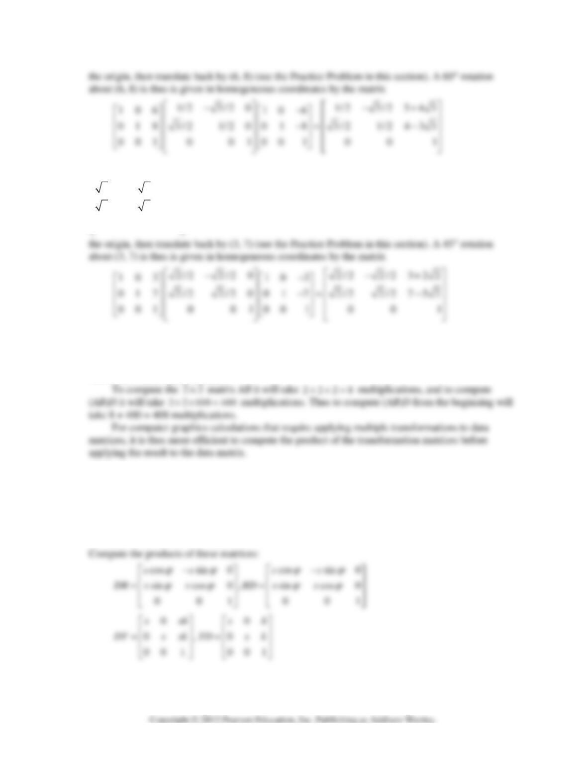
7. A 60° rotation about the origin is given in homogeneous coordinates by the matrix
1/ 2 3 / 2 0
3/2 1/2 0
⎡⎤
−
⎢⎥
⎢⎥
. To rotate about the point (6, 8), first translate by (–6, –8), then rotate about
140 CHAPTER 2 • Matrix Algebra
8. A 45° rotation about the origin is given in homogeneous coordinates by the matrix
2/2 2/2 0
2/2 2/2 0
001
⎡⎤
−
⎢⎥
⎢⎥
⎢⎥
⎢⎥
. To rotate about the point (3, 7), first translate by (–3, –7), then rotate about
9. To produce each entry in BD two multiplications are necessary. Since BD is a
2 100×
matrix, it will
take
2 2 100 400×× =
multiplications to compute BD. By the same reasoning it will take
22100×× =
400 multiplications to compute A(BD). Thus to compute A(BD) from the beginning will take
400 + 400 = 800 multiplications.
10. Let the transformation matrices in homogeneous coordinates for the dilation, rotation, and translation
be called respectively D, and R, and T. Then for some value of s,
ϕ
, h, and k,
00 cos sin 0 10
00,sincos0,01
001 0 0 1 001
sh
DsR T k
ϕϕ
ϕϕ
−
⎡⎤⎡ ⎤⎡⎤
⎢⎥⎢ ⎥⎢⎥
== =
⎢⎥⎢ ⎥⎢⎥
⎢⎥⎢ ⎥⎢⎥
⎣⎦⎣ ⎦⎣⎦
2.7 • Solutions 141
cos sin cos sin cos sin
hk h
ϕϕϕϕ ϕϕ
−− −
⎡⎤⎡⎤
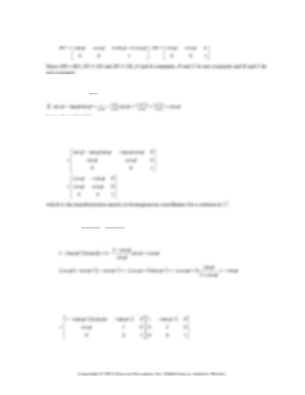
11. To simplify A
2
A
1
completely, the following trigonometric identities will be needed:
1.
sin
cos
tan cos cos sin
ϕ
ϕ
ϕϕ ϕ ϕ
−=−=−
Using these identities,
21
sec tan 0 1 0 0
010sincos0
001001
AA
ϕϕ
ϕϕ
−
⎡⎤⎡⎤
⎢⎥⎢⎥
=
⎢⎥⎢⎥
⎢⎥⎢⎥
⎣⎦⎣⎦
12. To simplify this product completely, the following trigonometric identity will be needed:
1cos sin
tan / 2 sin 1 cos
ϕϕ
ϕ
ϕϕ
−
==
+
This identity has two important consequences:
The product may be computed and simplified using these results:
1 tan / 2 0 1 0 0 1 tan / 2 0
010sin10010
001001001
ϕϕ
ϕ
−−
⎡⎤⎡⎤⎡⎤
⎢⎥⎢⎥⎢⎥
⎢⎥⎢⎥⎢⎥
⎢⎥⎢⎥⎢⎥
⎣⎦⎣⎦⎣⎦
142 CHAPTER 2 • Matrix Algebra
cos tan / 2 0 1 tan / 2 0
sin 1 0 0 1 0
0 01001
ϕϕ ϕ
ϕ
−−
⎡⎤⎡⎤
⎢⎥⎢⎥
=
⎢⎥⎢⎥
⎢⎥⎢⎥
⎣⎦⎣⎦
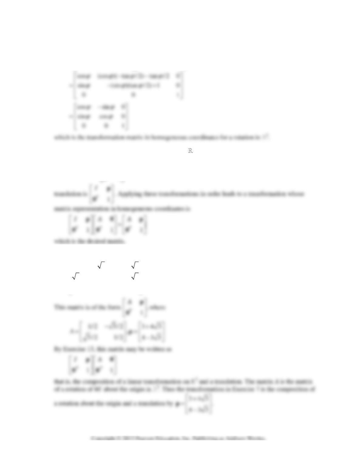
13. Consider first applying the linear transformation on
2
whose matrix is A, then applying a translation
by the vector p to the result. The matrix representation in homogeneous coordinates of the linear
transformation is ,
1
T
A
⎡⎤
⎢⎥
0
0
while the matrix representation in homogeneous coordinates of the
14. The matrix for the transformation in Exercise 7 was found to be
1/ 2 3 / 2 3 4 3
3/2 1/2 4 3 3
00 1
⎡⎤
−+
⎢⎥
−
⎢⎥
⎢⎥
⎢⎥
⎣⎦
2.7 • Solutions 143
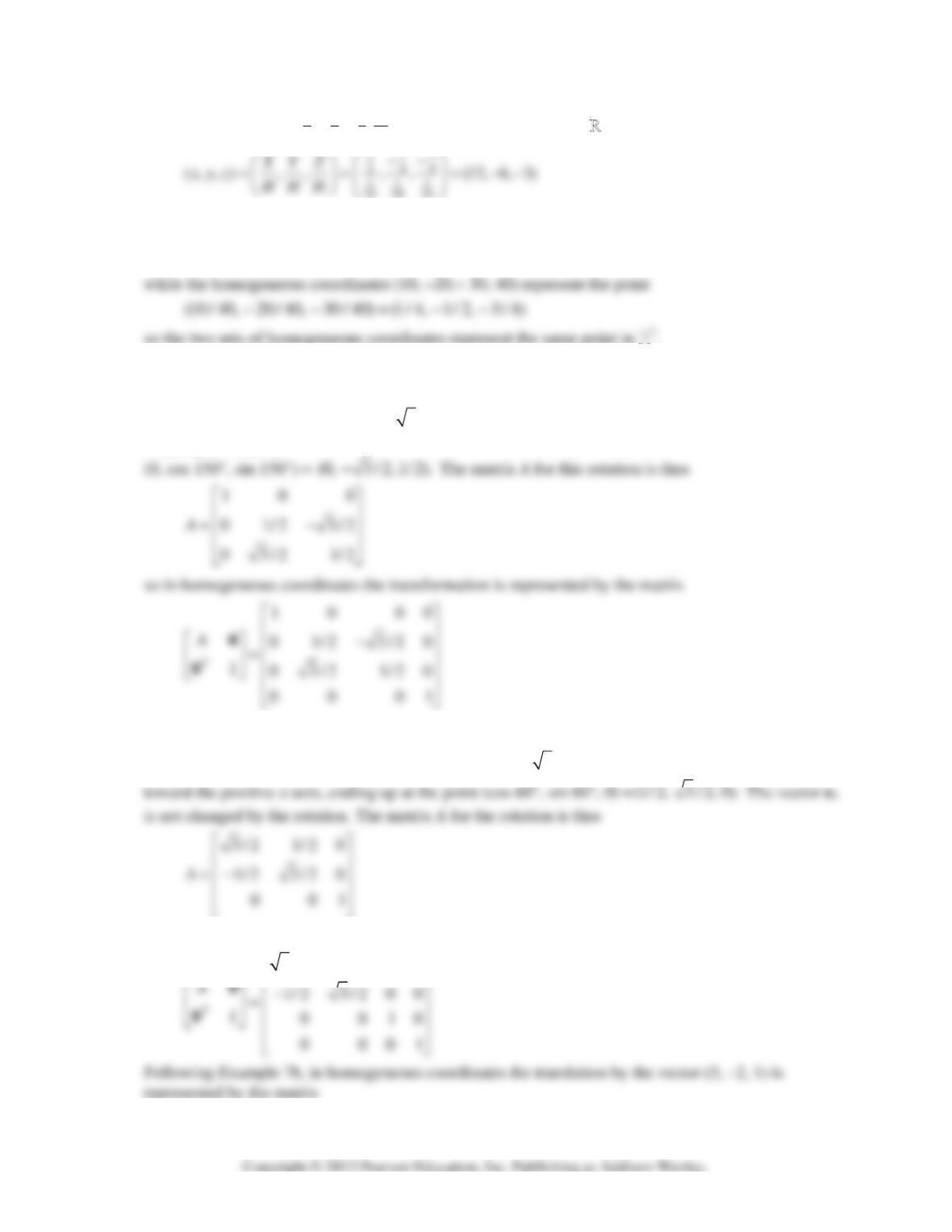
15. Since
1111
24824
(,,, )(, , ,),XYZH=−−
the corresponding point in
3
has coordinates
16. The homogeneous coordinates (1, –2, −3, 4) represent the point
(1/4, 2/4, 3/4) (1/4, 1/2, 3/4)−−= −−
.
17. Follow Example 7a by first constructing that
33×
matrix for this rotation. The vector e
1
is not
changed by this rotation. The vector e
2
is rotated 60° toward the positive z–axis, ending up at the
point (0, cos 60°, sin 60°) =
(0,1/2, 3/2).
The vector e
3
is rotated 60° toward the negative y–axis,
stopping at the point
18. First construct the
33×
matrix for the rotation. The vector e
1
is rotated 30° toward the negative y–
axis, ending up at the point (cos(–30)°, sin (–30)°, 0) =
( 3/2, 1/2,0).−
The vector e
2
is rotated 30°
so in homogeneous coordinates the rotation is represented by the matrix
3/2 1/200
⎡⎤
⎢⎥
144 CHAPTER 2 • Matrix Algebra
100 5
010 2
001 1
000 1
⎡⎤
⎢⎥
−
⎢⎥
⎢⎥
⎢⎥
⎢⎥
⎣⎦
Thus the complete transformation is represented in homogeneous coordinates by the matrix
⎢
⎢
⎢
⎢
⎢
⎣
10053/21/200 3/21/205
⎡
⎤⎡ ⎤
⎡⎤
19. Referring to the material preceding Example 8 in the text, we find that the matrix P that performs a
perspective projection with center of projection (0, 0, 10) is
10 00
⎡⎤
The homogeneous coordinates of the vertices of the triangle may be written as (4.2, 1.2, 4, 1), (6, 4,
2, 1), and (2, 2, 6, 1), so the data matrix for S is
4.2 6 2
1.2 4 2
⎡⎤
⎢⎥
and the data matrix for the transformed triangle is
1 0 0 0 4.2 6 2 4.2 6 2
⎡⎤⎡⎤⎡⎤
Finally, the columns of this matrix may be converted from homogeneous coordinates by dividing by
the final coordinate:
(4.2,1.2,0,.6) (4.2/.6,1.2/.6,0/.6) (7,2,0)
→=
20. As in the previous exercise, the matrix P that performs the perspective projection is
10 00
⎡⎤
2.8•Solutions145
The homogeneous coordinates of the vertices of the triangle may be written as (7, 3, –5, 1), (12, 8, 2,
1), and (1, 2, 1, 1), so the data matrix for S is
712 1
⎡⎤
⎢⎥
and the data matrix for the transformed triangle is
10 00 712 1 712 1
01 00 3 82 3 8 2
⎡⎤⎡⎤⎡⎤
⎢⎥⎢⎥⎢⎥
21. [M] Solve the given equation for the vector (R, G, B), giving
1
.61 .29 .15 2.2586 1.0395 .3473
RXX
−
−−
⎡⎤ ⎡ ⎤ ⎡ ⎤ ⎡ ⎤⎡ ⎤
22. [M] Solve the given equation for the vector (R, G, B), giving
1
.299 .587 .114 1.0031 .9548 .6179
RYY
−
⎡⎤ ⎡ ⎤⎡⎤ ⎡ ⎤⎡⎤
2.8 SOLUTIONS
Notes
: Cover this section only if you plan to skip most or all of Chapter 4. This section and the next
cover everything you need from Sections 4.1–4.6 to discuss the topics in Section 4.9 and Chapters 5–7
(except for the general inner product spaces in Sections 6.7 and 6.8). Students may use Section 4.2 for
review, particularly the Table near the end of the section. (The final subsection on linear transformations
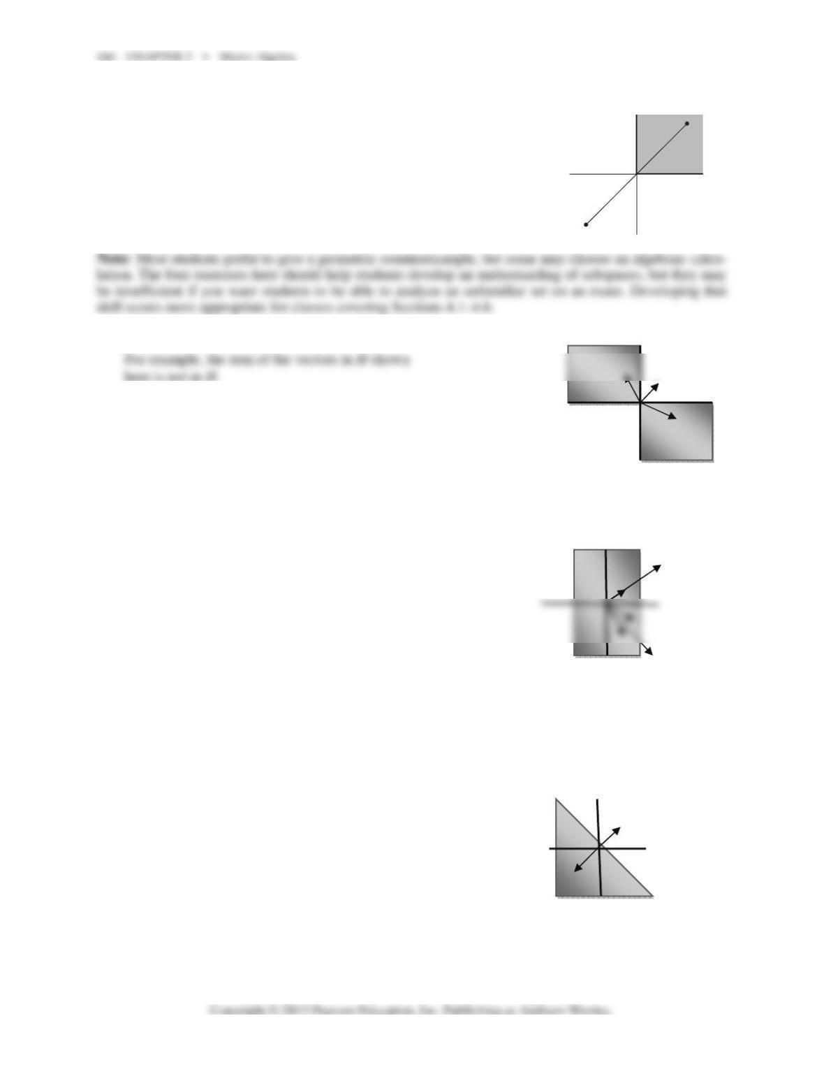
1. The set is closed under sums but not under multiplication
by a negative scalar. A counterexample to the subspace
condition is shown at the right.
2.The set is closed under scalar multiples but not sums.
3. No. The set is not closed under sums or scalar multiples. See the diagram.
4. No. The set is closed under sums, but not under multiplication by a
negative scalar.
u
(–1)u