2.3 • Solutions 107
41. [M] a. The exact solution of (3) is x
1
= 3.94 and x
2
= .49. The exact solution of (4) is x
1
= 2.90 and
x
2
= 2.00.
b. When the solution of (4) is used as an approximation for the solution in (3) , the error in using the
value of 2.90 for x
1
is about 26%, and the error in using 2.0 for x
2
is about 308%.
42. [M] MATLAB gives cond(A) 10, which is approximately 10
1
. If you make several trials with
MATLAB, which records 16 digits accurately, you should find that x and x
1
agree to at least 14 or 15
significant digits. So about 1 significant digit is lost. Here is the result of one experiment. The
vectors were all computed to the maximum 16 decimal places but are here displayed with only four
decimal places:
⎢
⎢
⎢
⎣
⎢
⎢
⎢
⎣
.9501
⎡
⎤
⎢
⎥
1.4219
−
⎡
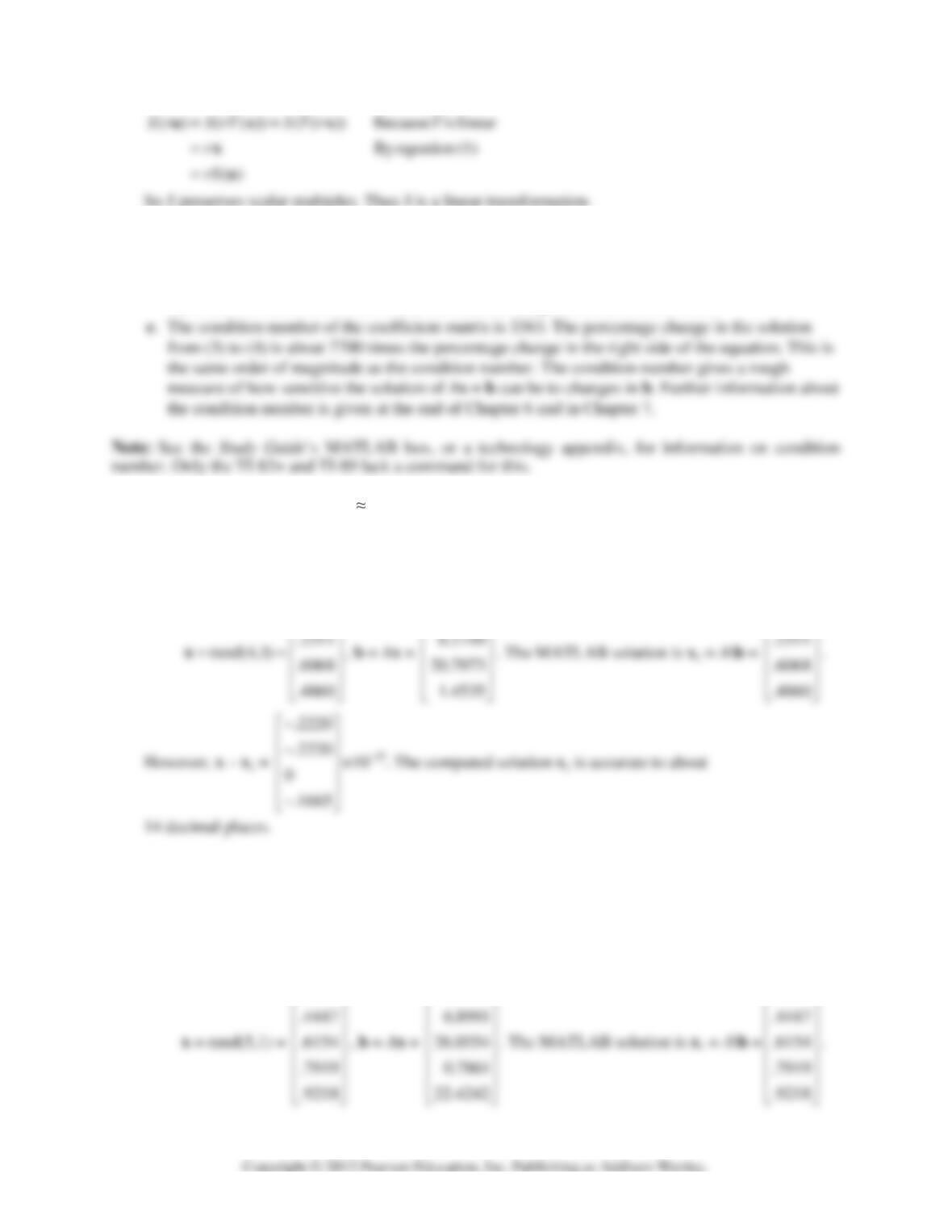
⎤
⎢
⎥
.9501
⎡⎤
⎢⎥
43. [M] MATLAB gives cond(A) = 69,000. Since this has magnitude between 10
4
and 10
5
, the
estimated accuracy of a solution of Ax = b should be to about four or five decimal places less than
the 16 decimal places that MATLAB usually computes accurately. That is, one should expect the
solution to be accurate to only about 11 or 12 decimal places. Here is the result of one experiment.
The vectors were all computed to the maximum 16 decimal places but are here displayed with only
four decimal places:
⎢
⎢
⎢
⎢
⎢
⎢
⎣
⎢
⎢
⎢
⎢
⎢
⎢
⎣
.8214
⎡
⎤
19.8965
⎡
⎤
.8214
⎡⎤
108 CHAPTER 2 • Matrix Algebra
1679
−
⎡⎤
44. [M] Solve Ax = (0, 0, 0, 0, 1). MATLAB shows that
5
cond( ) 4.8 10 .A≈×
Since MATLAB
45. [M] Some versions of MATLAB issue a warning when asked to invert a Hilbert matrix of order 12
or larger using floating-point arithmetic. The product AA
–1
should have several off-diagonal entries
Note:
All matrix programs supported by the Study Guide have data for Exercise 45, but only MATLAB
and Maple have a single command to create a Hilbert matrix.
Notes:
The Study Guide for Section 2.3 organizes the statements of the Invertible Matrix Theorem in a
table that imbeds these ideas in a broader discussion of rectangular matrices. The statements are arranged
in three columns: statements that are logically equivalent for any m×n matrix and are related to existence
concepts, those that are equivalent only for any n×n matrix, and those that are equivalent for any n×p
2.4 SOLUTIONS
Notes:
Partitioned matrices arise in theoretical discussions in essentially every field that makes use of
matrices. The Study Guide mentions some examples (with references).
Every student should be exposed to some of the ideas in this section. If time is short, you might omit
2.4 • Solutions 109
1. Apply the row-column rule as if the matrix entries were numbers, but for each product always write
the entry of the left block-matrix on the left.
2. Apply the row-column rule as if the matrix entries were numbers, but for each product always write
the entry of the left block-matrix on the left.
3. Apply the row-column rule as if the matrix entries were numbers, but for each product always write
the entry of the left block-matrix on the left.
4. Apply the row-column rule as if the matrix entries were numbers, but for each product always write
the entry of the left block-matrix on the left.
5. Compute the left side of the equation:
00
0000
ABI AIBX A BY
CXYCIXCY
++
⎡⎤⎡⎤⎡ ⎤
=
⎢⎥⎢⎥⎢ ⎥
++
⎣⎦⎣⎦⎣ ⎦
Since the (2, 1) blocks are equal, Z = C. Since the (1, 2) blocks are equal, BY = I. To proceed further,
assume that B and Y are square. Then the equation BY =I implies that B is invertible, by the IMT, and
–1
Note:
For simplicity, statements (j) and (k) in the Invertible Matrix Theorem involve square matrices
C and D. Actually, if A is n×n and if C is any matrix such that AC is the n×n identity matrix, then C must
be n×n, too. (For AC to be defined, C must have n rows, and the equation AC = I implies that C has n
6. Compute the left side of the equation:
00 000 0
XA XABXCXA
++
⎡⎤⎡⎤⎡ ⎤⎡ ⎤
110 CHAPTER 2 • Matrix Algebra
00 00
so that
00
XA I XA I
YA ZB ZC I YA ZB ZC I
==
⎡⎤⎡⎤
=
⎢⎥⎢⎥
++==
⎣⎦⎣⎦
To use the equality of the (1, 1) blocks, assume that A and X are square. By the IMT, the equation
XA =I implies that A is invertible and X = A
–1
. (See the boxed remark that follows the IMT.)
Similarly, if C and Z are assumed to be square, then the equation ZC = I implies that C is invertible,
by the IMT, and Z = C
–1
. Finally, use the (2, 1) blocks and right-multiplication by A
–1
:
7. Compute the left side of the equation:
0 0 00 00
AZ
XXABXZI
⎡⎤ ++ ++
⎡⎤ ⎡ ⎤
⎢⎥
Set this equal to the right side of the equation:
00
XA XZ I XA I XZ
==
⎡⎤⎡⎤
To use the equality of the (1, 1) blocks, assume that A and X are square. By the IMT, the equation XA
=I implies that A is invertible and X = A
–1
. (See the boxed remark that follows the IMT) Also, X is
invertible. Since XZ = 0, X
–1
XZ = X
–1
0 = 0, so Z must be 0. Finally, from the equality of the (2, 1)
8. Compute the left side of the equation:
00
000 00000
ABXY Z AXB AYB AZBI
IIXIYIZII
+++
⎡⎤⎡ ⎤⎡ ⎤
=
⎢⎥⎢ ⎥⎢ ⎥
++ +
⎣⎦⎣ ⎦⎣ ⎦
Set this equal to the right side of the equation:
To use the equality of the (1, 1) blocks, assume that A and X are square. By the IMT, the equation XA
=I implies that A is invertible and X = A
–1
. (See the boxed remark that follows the IMT. Since AY =
Note:
The Study Guide tells students, “Problems such as 5–10 make good exam questions. Remember to
9. Compute the left side of the equation:
11 12 11 21 31 12 22 32
00 0 0 0 0
IBBIBBBIBBB
++ ++
⎡⎤⎡⎤⎡ ⎤
Set this equal to the right side of the equation:
11 12 11 12
0
BBCC
AB B AB B C
⎡⎤⎡⎤
⎢⎥⎢⎥
++=
Since the (2,1) blocks are equal,
21 11 21 21 11 21
0and .AB B AB B+= =−
Since B
11
is invertible, right
multiplication by
11
11 21 21 11
gives .BABB
−−
=−
Likewise since the (3,1) blocks are equal,
31 11 31 31 11 31
0and .AB B AB B+= =−
Since B
11
is invertible, right multiplication by
10. Since the two matrices are inverses,
00 00 00
0000
00
II I
AI PI I
BDIQRI I
⎡⎤⎡⎤⎡⎤
⎢⎥⎢⎥⎢⎥
=
⎢⎥⎢⎥⎢⎥
⎢⎥⎢⎥⎢⎥
⎣⎦⎣⎦⎣⎦
Compute the left side of the equation:
Set this equal to the right side of the equation:
00 00
00 0
00
II
AP I I
BDPQ DR I I
⎡⎤⎡⎤
⎢⎥⎢⎥
+=
⎢⎥⎢⎥
⎢⎥⎢⎥
++ +
⎣⎦⎣⎦
11. a. True. See the subsection Addition and Scalar Multiplication.
12. a. False. The both AB and BA are defined.
13. You are asked to establish an if and only if statement. First, supose that A is invertible,
and let
1
DE
AFG
−
⎡⎤
=⎢⎥
⎣⎦
. Then
Since B is square, the equation BD = I implies that B is invertible, by the IMT. Similarly, CG = I
implies that C is invertible. Also, the equation BE = 0 imples that
1
E
B
−
=0 = 0. Similarly F = 0.
Thus
11
00
BDEB
−−
⎡⎤
⎡⎤⎡ ⎤
This proves that A is invertible only if B and C are invertible. For the “if ” part of the statement,
suppose that B and C are invertible. Then (*) provides a likely candidate for
1
A
−
which can be used
to show that A is invertible. Compute:
11
00 0 0
BB BB I
−−
⎡⎤⎡ ⎤
Since A is square, this calculation and the IMT imply that A is invertible. (Don’t forget this final
sentence. Without it, the argument is incomplete.) Instead of that sentence, you could add the
equation:
14. You are asked to establish an if and only if statement. First suppose that A is invertible. Example 5
shows that A
11
and A
22
are invertible. This proves that A is invertible only if A
11
A
22
are invertible. For
the if part of this statement, suppose that A
11
and A
22
are invertible. Then the formula in Example 5
provides a likely candidate for
1
A
−
which can be used to show that A is invertible . Compute:
⎣
1111
111
11 11 12 11 11 12 22 12 22
11 12 11 11 12 22
111 1
1
22 22 11 12 22 22 22
22 11
0()
0000()
0
AA A A A A A A A
AAAAAA
AAA AAAAA
A
−−−−
−−−
−−− −
−
⎡
⎤
+− +
⎡⎤
⎡⎤−
⎢
⎥
=
⎢⎥
⎢⎥ +− +
⎢
⎥
⎢⎥
⎣⎦
⎣⎦
15. The column-row expansions of G
k
and G
k+1
are:
2.4 • Solutions 113
and
T
GXX
=
16. Compute the right side of the equation:
11 11
11
11
11 11
11
0
00
00 0
AAY
A
I A IY IY
XA XA Y S
XA S
XI S I I
⎡
⎤
⎡⎤
⎡ ⎤⎡ ⎤⎡⎤ ⎡⎤
==
⎢
⎥
⎢⎥⎢ ⎥⎢ ⎥⎢⎥ ⎢⎥ +
⎣ ⎦⎣ ⎦⎣⎦ ⎣⎦
⎣⎦
⎣
⎦
Set this equal to the left side of the equation:
Since the (1, 2) blocks are equal,
11 12.AY A=
Since A
11
is invertible, left multiplication by
1
11
A
−
gives
17. Suppose that A and A
11
are invertible. First note that
000
0
II I
XI XI I
⎡⎤⎡ ⎤⎡⎤
=
⎢⎥⎢ ⎥⎢⎥
−
⎣⎦⎣ ⎦⎣⎦
and
are square, they are both invertible by the IMT. Equation (7) may be left multipled by
1
0I
XI
−
⎡⎤
⎢⎥
⎣⎦
and right multipled by
1
0
IY
I
−
⎡⎤
⎢⎥
⎣⎦
to find
114 CHAPTER 2 • Matrix Algebra
18. Since
[]
0
,WX=x
0
TTT
T
XXXX
⎡⎤ ⎡ ⎤
x
19. The matrix equation (8) in the text is equivalent to
() and
n
AsI B C−+= +=xu0 xuy
Rewrite the first equation as
() .
n
AsI B−=−xu
When
n
AsI−
is invertible,
20. The matrix in question is
n
m
ABCsI B
CI
−−
⎡⎤
⎢⎥
−
⎣⎦
21. a.
2
2
10 00
1010 10
2121 01
22 0(1)
A++
⎡⎤
⎡⎤⎡⎤ ⎡⎤
== =
⎢⎥
⎢⎥⎢⎥ ⎢⎥
−−−+−
⎣⎦⎣⎦ ⎣⎦
⎣⎦
22. Let C be any nonzero 2×2 matrix. Define
2
2
2
00
00
0
I
MI
CI
⎡
⎤
⎢
⎥
=
⎢
⎥
⎢
⎥
−
⎣
⎦
. Then
23. The product of two 1×1 “lower triangular” matrices is “lower triangular.” Suppose that for n = k, the
product of two k×k lower triangular matrices is lower triangular, and consider any (k+1)× (k+1)
matrices A
1
and B
1
. Partition these matrices as
11
,
TT
ab
AB
AB
⎡⎤ ⎡ ⎤
==
⎢⎥ ⎢ ⎥
⎣⎦ ⎣ ⎦
00
vw
where A and B are k×k matrices, v and w are in R
k
, and a and b are scalars. Since A
1
and B
1
are lower
triangular, so are A and B. Then
Note:
Exercise 23 is good for mathematics and computer science students. The solution of Exercise 23 in
the Study Guide shows students how to use the principle of induction. The Study Guide also has an
appendix on “The Principle of Induction,” at the end of Section 2.4. The text presents more applications
of induction in Section 3.2 and in the Supplementary Exercises for Chapter 3.
24. Let
100 0 1 0 0 0
110 0 1 1 0 0
,
111 0 0 1 1 0
111 1 0 11
nn
AB
⎡⎤⎡ ⎤
⎢⎥⎢ ⎥
−
⎢⎥⎢ ⎥
⎢⎥⎢ ⎥
==
−
⎢⎥⎢ ⎥
⎢⎥⎢ ⎥
⎢⎥⎢ ⎥
−
⎣⎦⎣ ⎦
“”
#% #%%
“”
.
By direct computation A
2
B
2
= I
2
. Assume that for n = k, the matrix A
k
B
k
is I
k
, and write
11
TT
⎡⎤ ⎡ ⎤
00
where v and w are in R
k
, v
T
= [1 1 ⋅ ⋅ ⋅ 1], and w
T
= [–1 0 ⋅ ⋅ ⋅ 0]. Then
11 1
1
11 1
TTT
TT T
k
kk k
T
kk k
kkk
B
AB I
AB I
AAB
++ +
⎡⎤
⎡⎤⎡ ⎤ ⎡ ⎤
++
== ==
⎢⎥
⎢⎥⎢ ⎥ ⎢ ⎥
++
⎢⎥
⎣⎦⎣ ⎦ ⎣ ⎦
⎣⎦
0w 0 0
00 0
vw 0
vwv0
The (2,1)-entry is 0 because v equals the first column of A
k
., and A
k
w is –1 times the first column of
A
k
. By the principle of induction, A
n
B
n
= I
n
for all n > 2. Since A
n
and B
n
are square, the IMT shows
that these matrices are invertible, and
1
.
nn
BA
−
=

2.3 • Solutions 101
D
–1
=
310
100 14 1
3013
−
⎡⎤
⎢⎥
−−
⎢⎥
⎢⎥
−
⎣⎦
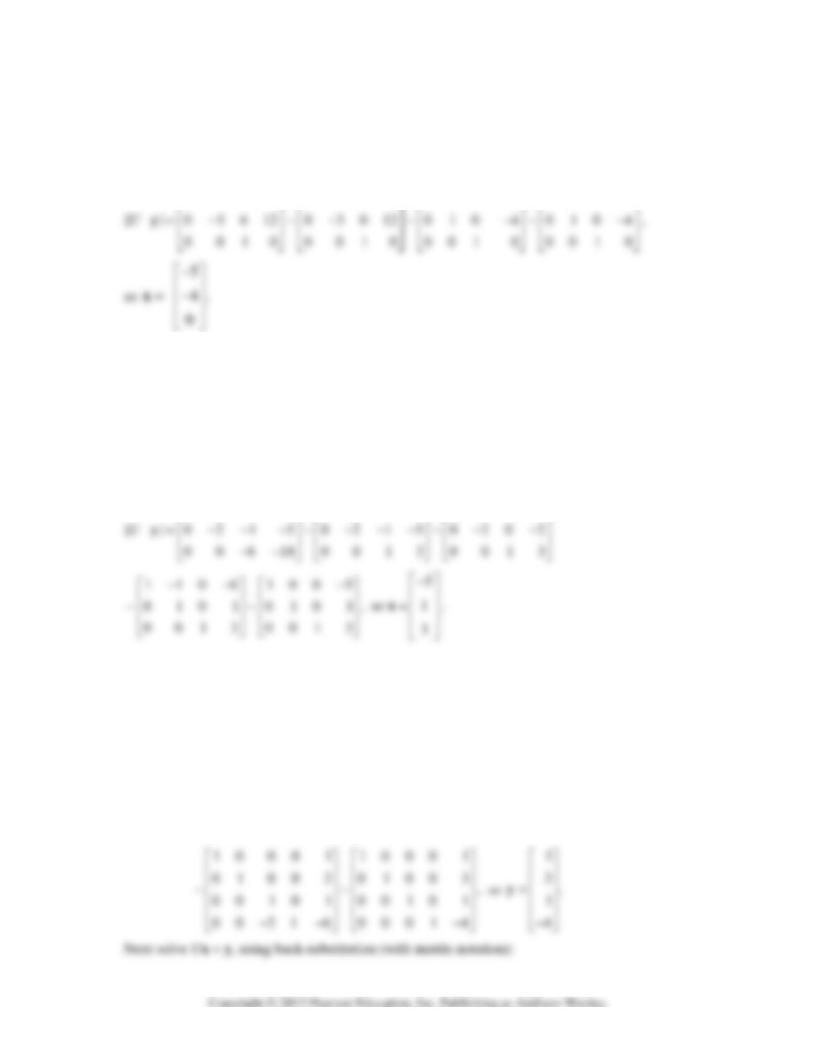
To find the forces (in pounds) required to produce a deflection of .04 cm at point 3, most students
will use technology to solve Df = (0, 0, .04) and obtain (0, –4/3, 4).
Here is another method, based on the idea suggested in Exercise 42. The first column of D
–1
lists the
41. To determine the forces that produce deflections of .07, .12, .16, and .12 cm at the four points on the
42. [M] To determine the forces that produce a deflection of .22 cm at the second point on the beam, use
technology to solve Df = y, where y = (0, .22, 0, 0). The forces at the four points are –10.476,
31.429,
–10.476, and 0 newtons, respectively (to three significant digits). These forces are .22 times the
entries in the second column of D
–1
. Reason: The transformation
1
D−
yy6
is linear, so the forces
required to produce a deflection of .22 cm at the second point are .22 times the forces required to
2.3 SOLUTIONS
Notes:
This section ties together most of the concepts studied thus far. With strong encouragement from
an instructor, most students can use this opportunity to review and reflect upon what they have learned,
and form a solid foundation for future work. Students who fail to do this now usually struggle throughout
the rest of the course. Section 2.3 can be used in at least three different ways.
(1) Stop after Example 1 and assign exercises only from among the Practice Problems and Exercises
(2) Include the subsection “Invertible Linear Transformations” in Section 2.3, if you covered Section
1.9. I do this when teaching “Course 1” because our mathematics and computer science majors take this
class. Exercises 29–40 support this material.
2.4 • Solutions 117
For [ j=10, j<=19, j++,
A [[ i,j ]] = B [[ i-4, j-9 ]] ] ]; Colon suppresses
output.
c. To create
0
0
T
A
B
A
⎡⎤
=⎢⎥
⎣⎦
with MATLAB, build B out of four blocks:
B = [A zeros(20,20); zeros(30,30) A’];
Another method: first enter B = A ; and then enlarge B with the command
27. a. [M] Construct A from four blocks, say C
11
, C
12
, C
21
, and C
22
, for example with C
11
a 30×30
matrix and C
22
a 20×20 matrix.
MATLAB: C11 = A(1:30, 1:30) + B(1:30, 1:30)
C12 = A(1:30, 31:50) + B(1:30, 31:50)
b. The algebra needed comes from block matrix multiplication:
11 12 11 12 11 11 12 21 11 12 12 22
21 22 21 22 21 11 22 21 21 12 22 22
AABB ABAB ABAB
AB AABB ABABABAB
++
⎡⎤⎡⎤⎡ ⎤
==
⎢⎥⎢⎥⎢ ⎥
++
⎣⎦⎣⎦⎣ ⎦
2.4 • Solutions 118
Example 5: Use equation (*) to find formulas for X, Y, and Z in terms of A, B, and C. Mention any
assumptions you make in order to produce the formulas.
00 0XI I
YZAB CI
⎡⎤⎡⎤⎡⎤
=
⎢⎥⎢⎥⎢⎥
⎣⎦⎣⎦⎣⎦
(*)
Solution:
This matrix equation provides four equations that can be used to find X, Y, and Z:
X + 0 = I, 0 = 0
The following counterexample shows that Z need not be square for the equation (*) above to be true.
100 0
1000 0 1000
0100
⎡⎤
⎡⎤ ⎡⎤
⎢⎥
⎢⎥ ⎢⎥
2.5 SOLUTIONS
Notes:
Modern algorithms in numerical linear algebra are often described using matrix factorizations.
For practical work, this section is more important than Sections 4.7 and 5.4, even though matrix
factorizations are explained nicely in terms of change of bases. Computational exercises in this section
emphasize the use of the LU factorization to solve linear systems. The LU factorization is performed
1.
100 37 2 7
1 1 0 , 0 2 1 , 5 . First, solve .
251 001 2
LU L
−− −
⎡⎤⎡⎤⎡⎤
⎢⎥⎢⎥⎢⎥
=− = − − = =
⎢⎥⎢⎥⎢⎥
⎢⎥⎢⎥⎢⎥
−−
⎣⎦⎣⎦⎣⎦
byb
2.5 • Solutions 119
100 7 7
010 2, so 2.
001 6 6
−−
⎡⎤⎡⎤
⎢⎥⎢⎥
∼−=−
⎢⎥⎢⎥
⎢⎥⎢⎥
⎣⎦⎣⎦
y
Next, solve Ux = y, using back-substitution (with matrix notation).
3727 3727 37019
−−− −−− − −
⎡⎤⎡⎤⎡⎤
3 70 19 300 9 100 3
~0 10 4 0 10 4 0 10 4
0 01 6 001 6 001 6
−−
⎡ ⎤⎡⎤⎡⎤
⎢ ⎥⎢⎥⎢⎥
∼ ∼
⎢ ⎥⎢⎥⎢⎥
⎢ ⎥⎢⎥⎢⎥
−−−
⎣ ⎦⎣⎦⎣⎦
, So x =
3
4.
6
⎡
⎤
⎢
⎥
⎢
⎥
⎢
⎥
−
⎣
⎦
To confirm this result, row reduce the matrix [A b]:
3727 3727 3727
−−− −−− −−−
⎡⎤⎡⎤⎡⎤
From this point the row reduction follows that of [U y] above, yielding the same result.
2.
100 264 2
210, 0 4 8, 4
011 002 6
LU
−
⎡⎤⎡ ⎤⎡⎤
⎢⎥⎢ ⎥⎢⎥
=− = − =−
⎢⎥⎢ ⎥⎢⎥
⎢⎥⎢ ⎥⎢⎥
−
⎣⎦⎣ ⎦⎣⎦
b
. First, solve Ly = b:
⎢
⎢
⎢
⎣
100 2 1002
⎡⎤⎡⎤
2
⎡
⎤
Next solve Ux = y, using back-substitution (with matrix notation):
2642 26014
[ ]0480 04024
0026 0013
U
−−
⎡⎤⎡⎤
⎢⎥⎢⎥
=− ∼ −
⎢⎥⎢⎥
⎢⎥⎢⎥
−−
⎣⎦⎣⎦
y
⎢
⎢
⎢
200 22 100 11
−−
⎡⎤⎡⎤
⎣⎦⎣⎦
11
−
⎡
⎤
⎣
⎦
To confirm this result, row reduce the matrix [A b]:
2642 2642
[ ] 4804 0480
0466 0026
A
−−
⎡⎤⎡⎤
⎢⎥⎢⎥
=− − ∼ −
⎢⎥⎢⎥
⎢⎥⎢⎥
−−
⎣⎦⎣⎦
b
From this point the row reduction follows that of [U y] above, yielding the same result.
100 2 42 6
−
⎡⎤⎡⎤⎡⎤
120 CHAPTER 2 • Matrix Algebra
1 006 1 00 6 100 6
[ ] 2100 01012 01012 ,
3116 01112 0010
L
⎡⎤⎡ ⎤⎡⎤
⎢⎥⎢ ⎥⎢⎥
=− ∼ ∼
⎢⎥⎢ ⎥⎢⎥
⎢⎥⎢ ⎥⎢⎥
−−−
⎣⎦⎣ ⎦⎣⎦
b
so
6
12 .
0
⎡
⎤
⎢
⎥
=
⎢
⎥
⎢
⎥
⎣
⎦
y
Next solve Ux = y, using back-substitution (with matrix notation):
2 426 2 406 200 10 100 5
−− −−
⎡⎤⎡⎤⎡⎤⎡⎤
4.
100 112 0
110, 021, 5
351 006 7
LU
−
⎡⎤⎡ ⎤⎡⎤
⎢⎥⎢ ⎥⎢⎥
==−−=−
⎢⎥⎢ ⎥⎢⎥
⎢⎥⎢ ⎥⎢⎥
−−
⎣⎦⎣ ⎦⎣⎦
b
. First, solve Ly = b:
1000 1000 100 0
[]11050105010 5 ,
3 517 0 517 00118
L
⎡⎤⎡⎤⎡⎤
⎢⎥⎢⎥⎢⎥
=−∼−∼−
⎢⎥⎢⎥⎢⎥
⎢⎥⎢⎥⎢⎥
−− −
⎣⎦⎣⎦⎣⎦
b
so
0
5 .
18
⎡⎤
⎢⎥
=−
⎢⎥
⎢⎥
−
⎣⎦
y
Next solve Ux = y, using back-substitution (with matrix notation):
112 0 1120 1106
−−−−
⎡⎤⎡⎤⎡⎤
5.
10 00 1 2 2 3 1
31 00 0 3 6 0 6
,, .
1010 0024 0
3421 0001 3
LU
−−−
⎡⎤⎡ ⎤⎡⎤
⎢⎥⎢ ⎥⎢⎥
−
⎢⎥⎢ ⎥⎢⎥
== =
⎢⎥⎢ ⎥⎢⎥
−
⎢⎥⎢ ⎥⎢⎥
−−
⎣⎦⎣ ⎦⎣⎦
b First solve Ly = b:
10 00 1 10 00 1
31 006 01 003
[] 10 100 00 10 1
34 21 3 04 21 6
L
⎡⎤⎡⎤
⎢⎥⎢⎥
⎢⎥⎢⎥
=∼
⎢⎥⎢⎥
−
⎢⎥⎢⎥
−− −
⎣⎦⎣⎦
b
2.5 • Solutions 121
12231 122011 1220 11
03603 0360 3 0360 3
[]
00241 002017 001017/2
00014 0001 4 0001 4
U
−−− −− − −− −
⎡⎤⎡⎤⎡ ⎤
⎢⎥⎢⎥⎢ ⎥
−−−
⎢⎥⎢⎥⎢ ⎥
=∼∼
⎢⎥⎢⎥⎢ ⎥
⎢⎥⎢⎥⎢ ⎥
−− −
⎣⎦⎣⎦⎣ ⎦
y
6.
1000 1320 1
2100 03012 2
, , .
3310 0020 1
5411 0001 2
LU
⎡⎤⎡⎤⎡⎤
⎢⎥⎢⎥⎢⎥
−−
⎢⎥⎢⎥⎢⎥
===
⎢⎥⎢⎥⎢⎥
−−−
⎢⎥⎢⎥⎢⎥
−−
⎣⎦⎣⎦⎣⎦
b First, solve Ly = b:
1000 1
0100 0
,
0010 4
⎢
⎣
⎡⎤
⎢⎥
⎢⎥
∼
⎢⎥
−
so
1
0.
4
⎡
⎤
⎢
⎥
⎢
⎥
=
⎢
⎥
−
y Next solve Ux = y, using back-substitution (with
00 0 1 3 00 01 3 0001 3
⎢⎥⎢⎥⎢⎥
⎣⎦⎣⎦⎣⎦
⎢
⎢
⎢
⎢
⎣
1000 33
⎡⎤
33
⎡
⎤
7. Place the first pivot column of
34
⎢⎥
−−
⎣⎦
into L, after dividing the column by 2 (the pivot), then add
8. Row reduce A to echelon form using only row replacement operations. Then follow the algorithm in
Example 2 to find L.
64 64
12 5 0 3
AU
⎡⎤⎡⎤
=∼ =
⎢⎥⎢⎥
−
⎣⎦⎣⎦
9.
31 2 312 312
90 4 032~032
9914 068 004
AU
⎡ ⎤⎡⎤⎡⎤
⎢ ⎥⎢⎥⎢⎥
=− − ∼ =
⎢ ⎥⎢⎥⎢⎥
⎢ ⎥⎢⎥⎢⎥
⎣ ⎦⎣⎦⎣⎦
2.5 • Solutions 123
1100
⎡⎤⎡⎤
10.
5 0 4 5 0 4 504
1025~023~023
10 10 16 0 10 24 0 0 9
AU
−−−
⎡⎤⎡⎤⎡⎤
⎢⎥⎢⎥⎢⎥
=− =
⎢⎥⎢⎥⎢⎥
⎢⎥⎢⎥⎢⎥
⎣⎦⎣⎦⎣⎦
[]
5
10 2
10 9
10
529
−
⎡⎤
⎢⎥
⎡⎤
⎢⎥
⎢⎥
⎢⎥
⎣⎦
⎣⎦
÷− ÷ ÷
11.
372 372 372
6194 050 050
3 23 055 005
AU
⎡ ⎤⎡⎤⎡⎤
⎢ ⎥⎢⎥⎢⎥
= ∼∼=
⎢ ⎥⎢⎥⎢⎥
⎢ ⎥⎢⎥⎢⎥
−−
⎣ ⎦⎣⎦⎣⎦
12. Row reduce A to echelon form using only row replacement operations. Then follow the algorithm in
Example 2 to find L. Use the last column of I
3
to make L unit lower triangular.
124 CHAPTER 2 • Matrix Algebra
232232232
4139 0 7 5 0 7 5
6 5 4 0 14 10 0 0 0
AU
⎡⎤⎡⎤⎡⎤
⎢⎥⎢⎥⎢⎥
=∼∼=
⎢⎥⎢⎥⎢⎥
⎢⎥⎢⎥⎢⎥
−
⎣⎦⎣⎦⎣⎦
13.
13 53 1 353 1353
1584 0 231 0231 No more pivots!
42 57 010155 0000
2475 0 231 0000
U
−− −− −−
⎡⎤⎡⎤⎡⎤
⎢⎥⎢⎥⎢⎥
−− − −
⎢⎥⎢⎥⎢⎥
∼∼=
⎢⎥⎢⎥⎢⎥
−− −
⎢⎥⎢⎥⎢⎥
−− −−
⎣⎦⎣⎦⎣⎦
14.
1315 1315 1315
520 6 31 0 51 6 0516
2 1 1 4 0 51 6 0000
1 7 1 7 010212 0000
AU
⎡⎤⎡⎤⎡⎤
⎢⎥⎢⎥⎢⎥
⎢⎥⎢⎥⎢⎥
=∼∼=
⎢⎥⎢⎥⎢⎥
−−−−
⎢⎥⎢⎥⎢⎥
−
⎣⎦⎣⎦⎣⎦
2.5 • Solutions 125
4
1
5
5
5
2
Use the last two columns of to make unit lower triangular.
10
1IL
⎡⎤
⎢⎥⎡⎤
⎢⎥⎢⎥
⎢⎥
−⎢⎥
⎢⎥⎢⎥
−⎣⎦
⎣⎦
15.
20 5 2 205 2 2052
6313303230323
4 9 16 17 0 9 6 13 0 0 0 4
AU
⎡⎤⎡⎤⎡⎤
⎢⎥⎢⎥⎢⎥
=− − − ∼ ∼ =
⎢⎥⎢⎥⎢⎥
⎢⎥⎢⎥⎢⎥
⎣⎦⎣⎦⎣⎦
16.
23 4 234 234
48 7 021 021
~~
6514 042 000
6912 000 000
8619 063 000
AU
−−−
⎡⎤⎡⎤⎡⎤
⎢⎥⎢⎥⎢⎥
−−
⎢⎥⎢⎥⎢⎥
⎢⎥⎢⎥⎢⎥
==
−
⎢⎥⎢⎥⎢⎥
−−
⎢⎥⎢⎥⎢⎥
⎢⎥⎢⎥⎢⎥
−
⎣⎦⎣⎦⎣⎦
126 CHAPTER 2 • Matrix Algebra
22
÷÷
17.
100 264
210, 0 4 8
011 002
LU
−
⎡⎤⎡ ⎤
⎢⎥⎢ ⎥
=− = −
⎢⎥⎢ ⎥
⎢⎥⎢ ⎥
−
⎣⎦⎣ ⎦
To find L
–1
, use the method of Section 2.2; that is, row
reduce [L I ]:
264100 260102
[ ]048010 040014
0 0 2001 0 0 200 1
UI
−−
⎡⎤⎡⎤
⎢⎥⎢⎥
=− ∼−
⎢⎥⎢⎥
⎢⎥⎢⎥
−−
⎣⎦⎣⎦
1
1/ 2 3/ 4 2
so 0 1 / 4 1 . Thus
001/2
U
−
−−
⎡⎤
⎢⎥
=− −
⎢⎥
⎢⎥
−
⎣⎦
18.
1
100 2 42
2 1 0 , 0 3 6 Tofind , row reduce[ ]:
311 001
LU LLI
−
−
⎡⎤⎡⎤
⎢⎥⎢⎥
=− = −
⎢⎥⎢⎥
⎢⎥⎢⎥
−
⎣⎦⎣⎦