r
2.1 SOLUTIONS
Notes:
The definition here of a matri
x
o
o
o
e
i
e
Exercises 23 and 24 are used in the
23–25 are mentioned in a footnote in S
e
can provide a transition to Section 2.2.
O
u
r
1. 201 4
2(2)
452 8
1
A−−
⎡⎤⎡
−=− =
⎢⎥⎢
−−
⎣⎦⎣
The product AC is not defined beca
u
rows of C. 12 35
21 14
CD ⎡⎤⎡⎤
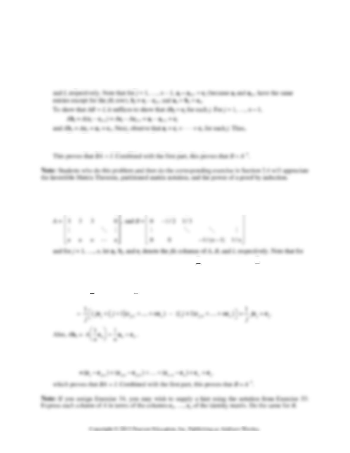
=⎢⎥⎢⎥
−−
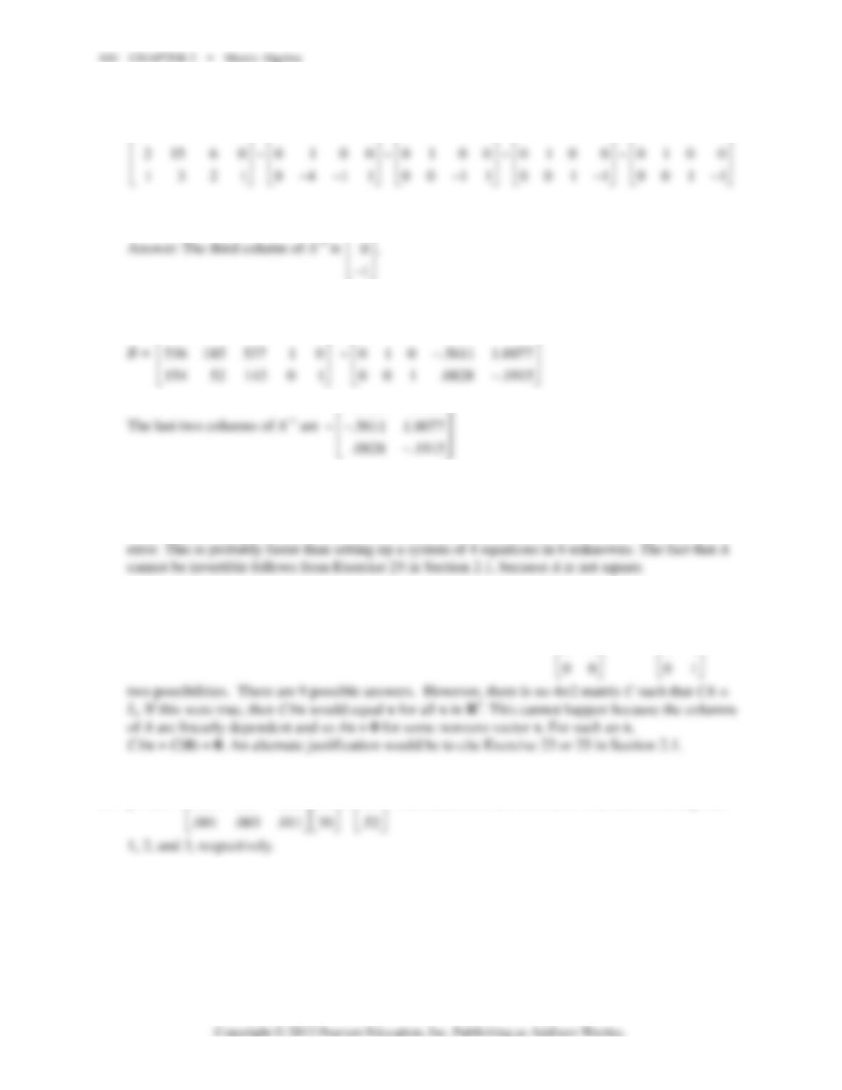
⎣⎦⎣⎦
computation, the row-column rule i
2. 201 75
33
452 14
AB −−
⎡⎤⎡
+= +
⎢⎥⎢
−−
⎣⎦⎣
The expression 2C – 3E is not defi
n
357 5 1
3
141 4 3
1
DB −
⎡⎤⎡ ⎤⎡
==
⎢⎥⎢ ⎥⎢
−−−−
⎣⎦⎣ ⎦⎣
u
u
u
u
r
x
product AB gives the proper view of AB for near
l
proof of the Invertible Matrix Theorem, in Section 2
.
e
ction 2.2. A class discussion of the solutions of Exe
r
O
r, these exercises could be assigned after starting Se
c
02
1
04
⎤
⎥
−⎦. Next, use B – 2A = B + (–2A):
u
se the number of columns of A does not match the n
u
13 2( 1) 15 2 4 1 13
23 1(1) 25 14 7 6
⋅+ − ⋅+ ⋅
⎡⎤⎡⎤
==
⎢⎥⎢⎥
−⋅ + − −⋅ +⋅ − −
⎣⎦⎣⎦
. For men
s probably easier to use than the definition.
1221015132315
2
3 4351229 7177
+−−+ −
⎤⎡ ⎤⎡
==
⎥⎢ ⎥⎢
−+−−− −−
⎦⎣ ⎦⎣
n
ed because 2C has 2 columns and –3E has only 1 col
u
3
7 51 3(5) 5(4) 31 5(3) 26 3
1
7 41 1(5) 4(4) 11 4(3) 3 1
⋅+⋅ − + − ⋅+ − −
⎤⎡
=
⎥⎢
⋅+⋅ −− + − −⋅+ − − −
⎦⎣
l
y all matrix
.
3. Exercises
r
cises 23–25
c
tion 2.2.
u
mber of
tal
2
⎤
⎥
⎦
u
mn.
512
113
−⎤
⎥
−⎦
88 CHAPTER 2 • Matrix Algebra
3.
2
3 0 2 5 32 0(5) 1 5
303 3 2 033(2) 35
IA −−−−
⎡⎤⎡ ⎤⎡ ⎤⎡ ⎤
−= − = =
⎢⎥⎢ ⎥⎢ ⎥⎢ ⎥
−−−−−
⎣⎦⎣ ⎦⎣ ⎦⎣ ⎦
4.
3
513 500 013
5 436050 426
312 005 313
AI
−−
⎡⎤⎡⎤⎡⎤
⎢⎥⎢⎥⎢⎥
−=− −− =−−−
⎢⎥⎢⎥⎢⎥
⎢⎥⎢⎥⎢⎥
−−−
⎣⎦⎣⎦⎣⎦
33
513 25515
(5 ) 5( ) 5 5 4 3 6 20 15 30
312 15510
IA IA A
−−
⎡⎤⎡ ⎤
⎢⎥⎢ ⎥
===− −=− −
⎢⎥⎢ ⎥
⎢⎥⎢ ⎥
−−
⎣⎦⎣ ⎦
, or
⎣⎦⎣⎦
5. a.
12
13 10 13 11
42
24 0, 24 8
23
53 26 53 19
AA
−−−
⎡⎤⎡⎤ ⎡⎤⎡⎤
−
⎡⎤ ⎡⎤
⎢⎥⎢⎥ ⎢⎥⎢⎥
====
⎢⎥ ⎢⎥
⎢⎥⎢⎥ ⎢⎥⎢⎥
−
⎣⎦ ⎣⎦
⎢⎥⎢⎥ ⎢⎥⎢⎥
−−−
⎣⎦⎣⎦ ⎣⎦⎣⎦
bb
6. a.
12
43 5 43 22
14
35 12, 35 22
32
01 3 01 2
AA
−− −
⎡⎤⎡⎤ ⎡⎤⎡⎤
⎡⎤ ⎡ ⎤
⎢⎥⎢⎥ ⎢⎥⎢⎥
=− = =− =−
⎢⎥ ⎢ ⎥
⎢⎥⎢⎥ ⎢⎥⎢⎥
−
⎣⎦ ⎣ ⎦
⎢⎥⎢⎥ ⎢⎥⎢⎥
−
⎣⎦⎣⎦ ⎣⎦⎣⎦
bb
2.1 • Solutions 89
43 4133443(2) 522
−⋅−⋅⋅−−−
⎡⎤ ⎡ ⎤⎡ ⎤
7. Since A has 3 columns, B must match with 3 rows. Otherwise, AB is undefined. Since AB has 7
columns, so does B. Thus, B is 3×7.
8. The number of rows of B matches the number of rows of BC, so B has 5 rows.
⎢
⎣
23 19 7183
k
−+
⎡⎤⎡⎤⎡ ⎤
19 2 3 7 12
−
⎡
⎤⎡ ⎤ ⎡ ⎤
3 6 1 1 21 21 3 6 3 5 21 21
−− − − −− − − −
⎡⎤⎡⎤⎡ ⎤⎡⎤⎡⎤⎡ ⎤
11.
123500 5 6 6
2 4 5 0 3 0 10 12 10
356002 151512
AD
⎡⎤⎡⎤⎡ ⎤
⎢⎥⎢⎥⎢ ⎥
==
⎢⎥⎢⎥⎢ ⎥
⎢⎥⎢⎥⎢ ⎥
⎣⎦⎣⎦⎣ ⎦
12. Consider B = [b
1
b
2
]. To make AB = 0, one needs Ab
1
= 0 and Ab
2
= 0. By inspection of A, a
suitable
⎡
⎢
⎣
13. Use the definition of AB written in reverse order: [Ab
1
⋅ ⋅ ⋅ Ab
p
] = A[b
1
⋅ ⋅ ⋅ b
p
]. Thus
[Qr
1
⋅ ⋅ ⋅ Qr
p
] = QR, when R = [r
1
⋅ ⋅ ⋅ r
p
].
14. By definition, UQ = U[q
1
⋅ ⋅ ⋅ q
4
] = [Uq
1
⋅ ⋅ ⋅ Uq
4
]. From Example 6 of Section 1.8, the vectorUq
1
lists the total costs (material, labor, and overhead) corresponding to the amounts of products B andC
15. a. False. See the definition of AB.
b. False. The roles of A and B should be reversed in the second half of the statement. See the box
3.
16. a. True. See the box after Example 4.
b. False. AB must be a 3×3 matrix, but the formula given here implies that it is a 3×1 matrix. The
plus signs should just be spaces (between columns). This is a common mistake.
17. Since
[]
12
311 ,
117AB A A
−−
⎡⎤
==
⎢⎥
⎣⎦
bb
the first column of B satisfies the equation
1.
6
A−
⎡⎤
=⎢⎥
⎣⎦
x Row
reduction:
[]
1
133 103
~~
351 012
AA −−
⎡
⎤⎡ ⎤
⎢
⎥⎢ ⎥
−
⎣
⎣
⎡
⎢
⎣
b. So b
1
=
3.
2
⎡
⎤
⎢
⎥
Similarly,
18. The third column of AB is also all zeros because Ab
3
= A0 = 0
19. (A solution is in the text). Write B = [b
1
b
2
b
3
]. By definition, the third column of AB is Ab
3
. By
20. The first two columns of AB are Ab
1
and Ab
2
. They are equal since b
1
and b
2
are equal.
Note:
The text answer for Exercise 21 is, “The columns of A are linearly dependent. Why?” The Study
22. If the columns of B are linearly dependent, then there exists a nonzero vector x such that Bx = 0.
23. If x satisfies Ax = 0, then CAx = C0 = 0 and so I
n
x = 0 and x = 0. This shows that the equation Ax = 0
has no free variables. So every variable is a basic variable and every column of A is a pivot column.
(A variation of this argument could be made using linear independence and Exercise 30 in Section
2.1 • Solutions 91
24. Write I
3
=[e
1
e
2
e
3
] and D = [d
1
d
2
d
3
]. By definition of AD, the equation AD = I
3
is equivalent
25. By Exercise 23, the equation CA = I
n
implies that (number of rows in A) > (number of columns), that
is, m > n. By Exercise 24, the equation AD = I
m
implies that (number of rows in A) < (number of
n
n
26. Take any b in R
m
. By hypothesis, ADb = I
m
b = b. Rewrite this equation as A(Db) = b. Thus, the
vector x = Db satisfies Ax = b. This proves that the equation Ax = b has a solution for each b in R
m
.
27. The product u
T
v is a 1×1 matrix, which usually is identified with a real number and is written
without the matrix brackets.
[]
32 5 3 2 5
T
a
babc
c
⎡⎤
⎢⎥
=− − =− + −
⎢⎥
⎢⎥
⎣⎦
uv ,
[]
3
2325
5
T
abc a b c
−
⎡⎤
⎢⎥
==−+−
⎢⎥
⎢⎥
−
⎣⎦
vu
28. Since the inner product u
T
v is a real number, it equals its transpose. That is,
29. The (i, j)-entry of A(B + C) equals the (i, j)-entry of AB + AC, because
111
()
nnn
ik kj kj ik kj ik kj
kkk
ab c ab ac
===
+= +
∑∑∑
30. The (i, j))-entries of r(AB), (rA)B, and A(rB) are all equal, because
nn n
31. Use the definition of the product I
m
A and the fact that I
m
x = x for x in R
m
.
32. Let e
and a
denote the jth columns of I
and A, respectively. By definition, the jth column of AI
is
33. The (i, j)-entry of (AB)
T
is the ( j, i)-entry of AB, which is
11ji jnni
ab ab+⋅⋅⋅+
34. Use Theorem 3(d), treating x as an n×1 matrix: (ABx)
T
= x
T
(AB)
T
= x
T
B
T
A
T
.
35. [M] The answer here depends on the choice of matrix program. For MATLAB, use the help
36. [M] The answer depends on the choice of matrix program. In MATLAB, the command
rand(5,6) creates a 5×6 matrix with random entries uniformly distributed between 0 and 1. The
command
37. [M] The equality AB = BA is very likely to be false for 4×4 matrices selected at random.
38. [M] (A + I)(A – I) – (A
2
– I) = 0 for all 5×5 matrices. However, (A + B)(A – B) – A
2
– B
2
is the zero
39. [M] The equality (A
T
+B
T
)=(A+B)
T
and (AB)
T
=B
T
A
T
should always be true, whereas (AB)
T
= A
T
B
T
is
very likely to be false for 4×4 matrices selected at random.
40. [M] The matrix S “shifts” the entries in a vector (a, b, c, d, e) to yield (b, c, d, e, 0). The entries in S
2
2.2 • Solutions 93
00100 00010 00001
⎡⎤⎡⎤⎡⎤
41. [M]
510
.3339 .3349 .3312 .333341 .333344 .333315
.3349 .3351 .3300 , .333344 .333350 .333306
.3312 .3300 .3388 .333315 .333306 .333379
AA
⎡⎤⎡ ⎤
⎢⎥⎢ ⎥
==
⎢⎥⎢ ⎥
⎢⎥⎢ ⎥
⎣⎦⎣ ⎦
The entries in A
20
all agree with .3333333333 to 8 or 9 decimal places. The entries in A
30
all agree
with .33333333333333 to at least 14 decimal places. The matrices appear to approach the matrix
1/3 1/3 1/3
⎡⎤
2.2 SOLUTIONS
Notes:
The text includes the matrix inversion algorithm at the end of the section because this topic is
popular. Students like it because it is a simple mechanical procedure. However, I no longer cover it in my
classes because technology is readily available to invert a matrix whenever needed, and class time is
better spent on more useful topics such as partitioned matrices. The final subsection is independent of the
inversion algorithm and is needed for Exercises 35 and 36.
1
86 4 6 2 3
1
−
−−
⎡⎤ ⎡ ⎤⎡ ⎤
1
32 5 2 52
1
−
−−
⎡⎤ ⎡ ⎤⎡ ⎤
1
73 33 33 1 1
11
−
−− −−
⎡⎤ ⎡⎤⎡⎤⎡ ⎤
94 CHAPTER 2 • Matrix Algebra
1
24 64 64 3/21
−
−−−−
5. The system is equivalent to Ax = b, where
86 2
and =
54 1
A
⎡
⎤⎡⎤
=
⎢
⎥⎢⎥
−
⎣
⎦⎣⎦
b, and the solution is
6. The system is equivalent to Ax = b, where
73 9
and
63 4
A−
⎡
⎤⎡⎤
==
⎢
⎥⎢⎥
−−
⎣
⎦⎣⎦
b, and the solution is x = A
–1
b.
To compute this by hand, the arithmetic is simplified by keeping the fraction 1/det(A) in front of the
7. a.
1
12 12 2 12 2 6 1
11
or
5 12 5 1 5 1 2.5 .5
112 2 5 2
−−− −
⎡⎤ ⎡ ⎤⎡ ⎤⎡ ⎤
==
⎢⎥ ⎢ ⎥⎢ ⎥⎢ ⎥
−− −
⋅−⋅
⎣⎦ ⎣ ⎦⎣ ⎦⎣ ⎦
x = A
–1
b
1
=
12 2 1 18 9
11
513 8 4
22
−− − −
⎡⎤⎡⎤⎡⎤⎡⎤
==
⎢⎥⎢⎥⎢⎥⎢⎥
−
⎣⎦⎣⎦⎣⎦⎣⎦
. Similar calculations give
b. [A b
1
b
2
b
3
b
4
] =
12 1 123
512 3 5 6 5
−
⎡⎤
⎢⎥
−
⎣⎦
⎡
⎢
⎣
12 1 1 2 3 12 1 1 2 3
−−
Note:
The Study Guide also discusses the number of arithmetic calculations for this Exercise 7, stating
that when A is large, the method used in (b) is much faster than using A
–1
.
8. Left-multiply each side of A = PBP
–1
by P
–1
:
P
–1
A = P
–1
PBP
–1
, P
–1
A = IBP
–1
, P
–1
A = BP
–1
9. a. True, by definition of invertible.
2.2 • Solutions 95
b. False. See Theorem 6(b).
10. a. False. The last part of Theorem 7 is misstated here.
b. True, by Theorem 6(a).
11. (The proof can be modeled after the proof of Theorem 5.) The n×p matrix B is given (but is
arbitrary). Since A is invertible, the matrix A
–1
B satisfies AX = B, because A(A
–1
B) = A A
–1
B = IB =
B. To show this solution is unique, let X be any solution of AX = B. Then, left-multiplication of each
12. Left-multiply each side of the equation AD = I by A
–1
to obtain
13. Left-multiply each side of the equation AB = AC by A
–1
to obtain
14. Right-multiply each side of the equation (B – C)D = 0 by D
–1
to obtain
15. If you assign this exercise, consider giving the following Hint: Use elementary matrices and imitate
the proof of Theorem 7. The solution in the Instructor’s Edition follows this hint. Here is another
solution, based on the idea at the end of Section 2.2.
Write B = [b
1
⋅ ⋅ ⋅ b
p
] and X = [u
1
⋅ ⋅ ⋅ u
p
]. By definition of matrix multiplication,
Since A is the coefficient matrix in each system, these systems may be solved simultaneously,
placing the augmented columns of these systems next to A to form [A b
1
⋅ ⋅ ⋅ b
p
] = [A B]. Since A
is invertible, the solutions u
1
, …, u
p
are uniquely determined, and [A b
1
⋅ ⋅ ⋅ b
p
] must row reduce to
16. Let C = AB. Then CB
–1
= ABB
–1
, so CB
–1
= AI = A. This shows that A is the product of invertible
matrices and hence is invertible, by Theorem 6.
17. The box following Theorem 6 suggests what the inverse of ABC should be, namely, C
–1
B
–1
A
–1
. To
verify that this is correct, compute:
18. Right-multiply each side of AB = BC by B
–1
:
19. Unlike Exercise 18, this exercise asks two things, “Does a solution exist and what is it?” First, find
CC
–1
(A + X)B
–1
= CI, I(A + X)B
–1
= C, (A + X)B
–1
B = CB, (A + X)I = CB
Expand the left side and then subtract A from both sides:
Note:
The Study Guide suggests that students ask their instructor about how many details to include in
their proofs. After some practice with algebra, an expression such as CC
–1
(A + X)B
–1
could be simplified
20. a. Left-multiply both sides of (A – AX)
–1
= X
–1
B by X to see that B is invertible because it is the
(which applies because X
–1
and B are invertible):
Then A = AX + B
–1
X = (A + B
–1
)X. The product (A + B
–1
)X is invertible because A is invertible.
Since X is known to be invertible, so is the other factor, A + B
–1
, by Exercise 16 or by an
Note:
This exercise is difficult. The algebra is not trivial, and at this point in the course, most students
will not recognize the need to verify that a matrix is invertible.
21. Suppose A is invertible. By Theorem 5, the equation Ax = 0 has only one solution, namely, the zero
22. Suppose A is invertible. By Theorem 5, the equation Ax = b has a solution (in fact, a unique solution)
23. Suppose A is n×n and the equation Ax = 0 has only the trivial solution. Then there are no free
24. If the equation Ax = b has a solution for each b in R
n
, then A has a pivot position in each row, by
Theorem 4 in Section 1.4. Since A is square, the pivots must be on the diagonal of A. It follows that A
25. Suppose
ab
Acd
=
⎡⎤
⎢⎥
⎣⎦
and ad – bc = 0. If a = b = 0, then examine
1
2
00 0
0
x
x
cd
⎡⎤
⎡
⎤⎡⎤
=
⎢⎥
⎢
⎥⎢⎥
⎣
⎦⎣⎦
⎣⎦
This has the
solution x
1
=
d
c
⎡⎤
⎢⎥
−
⎣⎦
. This solution is nonzero, except when a = b = c = d. In that case, however, A is
26.
0
0
d b a b da bc
cacd cbad
−−
⎡⎤⎡⎤⎡ ⎤
=
⎢⎥⎢⎥⎢ ⎥
−−+
⎣⎦⎣⎦⎣ ⎦
. Divide both sides by ad – bc to get CA = I.
27. a. Interchange A and B in equation (1) after Example 6 in Section 2.1: row
i
(BA) = row
i
(B)⋅A. Then
replace B by the identity matrix: row
i
(A) = row
i
(IA) = row
i
(I)⋅A.
b. Using part (a), when rows 1 and 2 of A are interchanged, write the result as
22 2
row ( ) row ( ) row ( )
AIAI
⋅
⎡⎤⎡ ⎤⎡⎤
c. Using part (a), when row 3 of A is multiplied by 5, write the result as
row ( ) row ( ) row ( )
AIAI
⋅
⎡⎤⎡ ⎤⎡⎤
28. When row 2 of A is replaced by row
2
(A) – 3⋅row
1
(A), write the result as
11
row ( ) row ( )
AIA
⋅
⎡⎤⎡ ⎤
2
2
1
29.
1 3 10 1 3 10 10 31 10 3 1
[] ~ ~ ~
4 901 0 3 41 03 41 01 4/31/3
AI −− − −
⎡⎤⎡⎤⎡⎤⎡ ⎤
=⎢⎥⎢⎥⎢⎥⎢ ⎥
−−−−
⎣⎦⎣⎦⎣⎦⎣ ⎦
30.
36 1 0 121/30 1 2 1/3 0
[] ~ ~
47 0 1 47 0 1 0 1 4/3 1
AI ⎡⎤⎡ ⎤⎡ ⎤
=⎢⎥⎢ ⎥⎢ ⎥
−−
⎣⎦⎣ ⎦⎣ ⎦
31.
102100 10 2 100
[]314010~012310
2 3 4001 0 3 8 2 0 1
AI
−−
⎡⎤⎡ ⎤
⎢⎥⎢ ⎥
=− −
⎢⎥⎢ ⎥
⎢⎥⎢ ⎥
−−−
⎣⎦⎣ ⎦
10 2100 100 831
~0 1 2 3 1 0~0 1 0 10 4 1
−
⎡⎤⎡⎤
⎢⎥⎢⎥
−
32.
121100 121100
[]473010~011410
AI
−−
⎡⎤⎡⎤
⎢⎥⎢⎥
=− − −
⎢⎥⎢⎥
2.2 • Solutions 99
33. Let B =
100 0
110 0
011
00 11
⎡⎤
⎢⎥
−
⎢⎥
⎢⎥
−
⎢⎥
⎢⎥
⎢⎥
−
⎣⎦
, and for j = 1, …, n, let a
j
, b
j
, and e
j
denote the jth columns of A, B,
Ba
j
= B(e
j
+ ⋅ ⋅ ⋅ + e
n
) = b
j
+ ⋅ ⋅ ⋅ + b
n
= (e
j
– e
j+1
) + (e
j+1
– e
j+2
) + ⋅ ⋅ ⋅ + (e
n–1
– e
n
) + e
n
= e
j
34. Let
100 0 1 0 0 0
220 0 1 1/2 0
⎡⎤⎡ ⎤
⎢⎥⎢ ⎥
−
j = 1, …, n–1, a
j
= je
j
+(j+1)e
j+1
⋅ ⋅ ⋅ +n e
n
, a
n
= n e
n
, b
j
=
1
1()
jj
j
+
−ee , and
1.
nn
n
=be
To show that AB = I, it suffices to show that Ab
j
= e
j
for each j. For j = 1, …, n–1,
Ab
j
= A
1
1()
jj
j
+
⎛⎞
−
⎜⎟
⎝⎠
ee =
1
1()
jj
j
+
−aa
Moreover,
()
jj1 1
1B ( 1)
jnjjn
BjB j nBj j n
++
=++ ++ =++ ++ae e eb b b……
35. Row reduce [A e
3
]:
1 7 3 0 1 7 3 0 17 30 103 0 100 3
−−−
⎡⎤⎡⎤⎡⎤⎡⎤⎡⎤
3
⎡⎤
36. [M] Write B = [A F], where F consists of the last two columns of I
3
, and row reduce:
25 9 27 0 0
−−−
⎡⎤
1 0 0 .1126 .1559
−
⎡⎤
.1126 .1559
−
⎡⎤
37. There are many possibilities for C, but C =
11 1
11 0
−
⎡
⎤
⎢
⎥
−
⎣
⎦
is the only one whose entries are 1, –1,
and 0. With only three possibilities for each entry, the construction of C can be done by trial and
38. Write AD = A[d
1
d
2
] = [Ad
1
Ad
2
]. The structure of A shows that D =
11
01
00
⎢
⎣
⎡
⎤
⎢
⎥
⎢
⎥
⎢
⎥
and D =
10
11
11
⎡⎤
⎢⎥
⎢⎥
⎢⎥
are
39. y = Df =
.011 .003 .001 40 .62
.003 .009 .003 50 .66
⎡⎤⎡⎤⎡⎤
⎢⎥⎢⎥⎢⎥
=
. The deflections are .62 in., .66 in., and .52 in. at points
40. [M] The stiffness matrix is D
–1
. Use an “inverse” command to produce
2.3 • Solutions 101
D
–1
=
310
100 14 1
3013
−
⎡⎤
⎢⎥
−−
⎢⎥
⎢⎥
−
⎣⎦
To find the forces (in pounds) required to produce a deflection of .04 cm at point 3, most students
41. To determine the forces that produce deflections of .07, .12, .16, and .12 cm at the four points on the
42. [M] To determine the forces that produce a deflection of .22 cm at the second point on the beam, use
technology to solve Df = y, where y = (0, .22, 0, 0). The forces at the four points are –10.476,
31.429,
Note:
The Study Guide suggests using gauss, swap, bgauss, and scale to reduce [A I]
2.3 SOLUTIONS
Notes:
This section ties together most of the concepts studied thus far. With strong encouragement from
an instructor, most students can use this opportunity to review and reflect upon what they have learned,
and form a solid foundation for future work. Students who fail to do this now usually struggle throughout
the rest of the course. Section 2.3 can be used in at least three different ways.
(1) Stop after Example 1 and assign exercises only from among the Practice Problems and Exercises
(2) Include the subsection “Invertible Linear Transformations” in Section 2.3, if you covered Section
(3) Skip the linear transformation material here, but discusses the condition number and the
Numerical Notes. Assign exercises from among 1–28 and 41–45, and perhaps add a computer project on
102 CHAPTER 2 • Matrix Algebra
8).
1. The columns of the matrix
57
36
⎡⎤
⎢⎥
−−
⎣⎦
are not multiples, so they are linearly independent. By (e) in
the IMT, the matrix is invertible. Also, the matrix is invertible by Theorem 4 in Section 2.2 because
the determinant is nonzero.
3. Row reduction to echelon form is trivial because there is really no need for arithmetic calculations:
300 300 500
340~040~040
⎡ ⎤⎡⎤⎡⎤
⎢ ⎥⎢⎥⎢⎥
−− − −
The 3×3 matrix has 3 pivot positions and hence is
4. The matrix
514
000
−
⎡⎤
⎢⎥
cannot row reduce to the identity matrix since it already contains a row of
5. The matrix
30 3
20 4
40 7
−
⎡⎤
⎢⎥
⎢⎥
⎢⎥
−
⎣⎦
obviously has linearly dependent columns (because one column is zero),
6.
136 13 6 136 13 6
043~04 3~043~04 3
−− − − −− − −
⎡⎤⎡⎤⎡⎤⎡⎤
⎢⎥⎢⎥⎢⎥⎢⎥
7.
1301 1301 1301
3583 0480 0480
~~
−− −− −−
⎡⎤⎡⎤⎡⎤
⎢⎥⎢⎥⎢⎥
−− −
⎢⎥⎢⎥⎢⎥
2.3 • Solutions 103
8. The 4×4 matrix
3474
0028
0001
⎡⎤
⎢⎥
⎢⎥
⎣⎦
is invertible because it has four pivot positions, by (c) of the IMT.
4037 1000
6999 0100
−−
⎡⎤⎡⎤
⎢⎥⎢⎥
−
The 4×4 matrix is invertible because it has four pivot positions, by (c) of the IMT.
10. [M]
531 7 9 5 3 1 7 9
6 4 2 8 8 0 .4 .8 .4 18.8
~
75310 9 0 .81.6 .2 3.6
9 6 4 9 5 0 .6 2.2 21.6 21.2
⎡⎤⎡ ⎤
⎢⎥⎢ ⎥
−−−
⎢⎥⎢ ⎥
⎢⎥⎢ ⎥
−
⎢⎥⎢ ⎥
−− − −
⎢⎥⎢ ⎥
11. a. True, by the IMT. If statement (d) of the IMT is true, then so is statement (b).
b. True. If statement (h) of the IMT is true, then so is statement (e).
c. False. Statement (g) of the IMT is true only for invertible matrices.
12. a. True. If statement (k) of the IMT is true, then so is statement ( j). Use the first box after the IMT.
b. False. Notice that (i) if the IMT uses the work onto rather than the word into.
c. True. If statement (e) of the IMT is true, then so is statement (h).
13. If a square upper triangular n×n matrix has nonzero diagonal entries, then because it is already in
14. If A is lower triangular with nonzero entries on the diagonal, then these n diagonal entries can be
used as pivots to produce zeros below the diagonal. Thus A has n pivots and so is invertible, by the
IMT. If one of the diagonal entries in A is zero, A will have fewer than n pivots and hence be
singular.
Notes:
For Exercise 14, another correct analysis of the case when A has nonzero diagonal entries is to
apply the IMT (or Exercise 13) to A
T
. Then use Theorem 6 in Section 2.2 to conclude that since A
T
is
invertible so is its transpose, A. You might mention this idea in class, but I recommend that you not spend
15. Part (h) of the IMT shows that a 4×4 matrix cannot be invertible when its columns do not span R
4
.
16. If A is invertible, so is A
T
, by (l) of the IMT. By (e) of the IMT applied to A
T
, the columns of A
T
are
linearly independent.
7
20. By (g) of the IMT, A is invertible. Hence, each equation Ax = b has a unique solution, by Theorem 5
in Section 2.2. This fact was pointed out in the paragraph following the proof of the IMT.
22. By the box following the IMT, E and F are invertible and are inverses. So FE = I = EF, and so E and
F commute.
24. Statement (b) of the IMT is false for G, so statements (e) and (h) are also false. That is, the columns
of G are linearly dependent and the columns do not span R
n
.
25. Suppose that A is square and AB = I. Then A is invertible, by the (k) of the IMT. Left-multiplying
each side of the equation AB = I by A
–1
, one has
A
2.3 • Solutions 105
26. If the columns of A are linearly independent, then since A is square, A is invertible, by the IMT. So
27. Let W be the inverse of AB. Then ABW = I and A(BW) = I. Since A is square, A is invertible, by (k) of
the IMT.
29. Since the transformation
A
xx
is one-to-one, statement (f) of the IMT is true. Then (i) is also true
30. Since the transformation Axx is not one-to-one, statement (f) of the IMT is false. Then (i) is also
31. Since the equation Ax = b has a solution for each b, the matrix A has a pivot in each row (Theorem 4
in Section 1.4). Since A is square, A has a pivot in each column, and so there are no free variables in
32. If Ax = 0 has only the trivial solution, then A must have a pivot in each of its n columns. Since A is
square (and this is the key point), there must be a pivot in each row of A. By Theorem 4 in Section
33. (Solution in Study Guide) The standard matrix of T is
59
,
47
A
−
⎡
⎤
=
⎢
⎥
−
⎣
⎦
which is invertible because
det A ≠ 0. By Theorem 9, the transformation T is invertible and the standard matrix of T
–1
is A
–1
.
⎡
⎢
⎣
106 CHAPTER 2 • Matrix Algebra
34. The standard matrix of T is
28
,
27
A
−
⎡⎤
=⎢⎥
−
⎣⎦
which is invertible because det A = -2 ≠ 0. By Theorem
35. (Solution in Study Guide) To show that T is one-to-one, suppose that T(u) = T(v) for some vectors u
and v in R
n
. Then S(T(u)) = S(T(v)), where S is the inverse of T. By Equation (1), u = S(T(u)) and
S(T(v)) = v, so u = v. Thus T is one-to-one. To show that T is onto, suppose y represents an arbitrary
36. Let A be the standard matrix of T. By hypothesis, T is not a one-to-one mapping. So, by Theorem 12
37. Let A and B be the standard matrices of T and U, respectively. Then AB is the standard matrix of the
mapping (())TUxx, because of the way matrix multiplication is defined (in Section 2.1). By
hypothesis, this mapping is the identity mapping, so AB = I. Since A and B are square, they are
.
38. Given any v in R
n
, we may write v = T(x) for some x, because T is an onto mapping. Then, the
39. If T maps R
n
onto R
n
, then the columns of its standard matrix A span R
n
, by Theorem 12 in Section
1.9. By the IMT, A is invertible. Hence, by Theorem 9 in Section 2.3, T is invertible, and A
–1
is the
40. Given u, v in
n
, let x = S(u) and y = S(v). Then T(x)=T(S(u)) = u and T(y) = T(S(v)) = v, by
equation (2). Hence