1.1 SOLUTIONS
Notes:
The key exercises are 7 (or 11 or 12), 19–22, and 25. For brevity, the symbols R1, R2,…, stand
for row 1 (or equation 1), row 2 (or equation 2), and so on. Additional notes are at the end of the section.
1.
12
12
57
27 5
xx
xx
+=
−− =−
157
275
⎡
⎤
⎢
⎥
−−−
⎣
⎦
⎢
⎣
⎡
⎢
⎣
⎡
⎢
⎣
12
57
xx
+=
157
⎡
⎤
2.
12
12
36 3
57 10
xx
xx
+=−
+=
36 3
5710
−
⎡
⎤
⎢
⎥
⎣
⎦
Scale R1 by 1/3 and obtain:
12
12
21
57 10
xx
xx
+=−
+=
12 1
5710
−
⎡
⎤
⎢
⎥
⎣
⎦
⎡
⎢
⎣
⎡
⎢
⎣
⎡
⎢
⎣
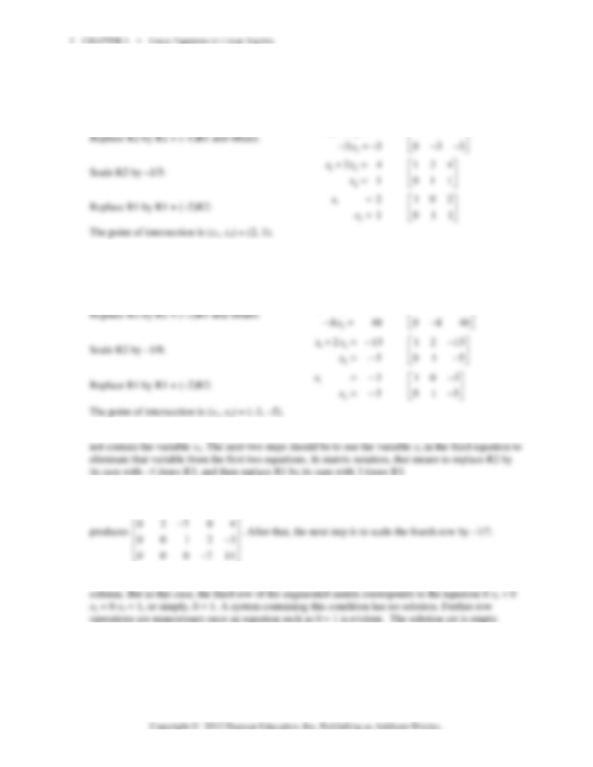
3. The point of intersection satisfies the system of two linear equations:
12
12
24
1
xx
xx
+=
−=
124
111
⎡⎤
⎢⎥
−
⎣⎦
⎢
⎣
⎡
⎢
⎣
⎡
⎢
⎣
12
24
xx
+=
124
⎡
⎤
4. The point of intersection satisfies the system of two linear equations:
12
12
213
32 1
xx
xx
+=−
−=
1213
32 1
−
⎡⎤
⎢⎥
−
⎣⎦
⎢
⎣
⎡
⎢
⎣
⎡
⎢
⎣
12
213
xx
+=−
1213
−
⎡
⎤
5. The system is already in “triangular” form. The fourth equation is x
4
= –5, and the other equations do
6. One more step will put the system in triangular form. Replace R4 by its sum with –4 times R3, which
164 0 1
−−
⎡⎤
7. Ordinarily, the next step would be to interchange R3 and R4, to put a 1 in the third row and third
1.1 • Solutions 3
8. The standard row operations are:
1 5400 1 5400 1 5400 1 5400
01010010100100001000
~~~
0 0010 00010
−−−−
⎡⎤⎡⎤⎡⎤⎡⎤
⎢⎥⎢⎥⎢⎥⎢⎥
⎢⎥⎢⎥⎢⎥⎢⎥
⎣⎦⎣⎦
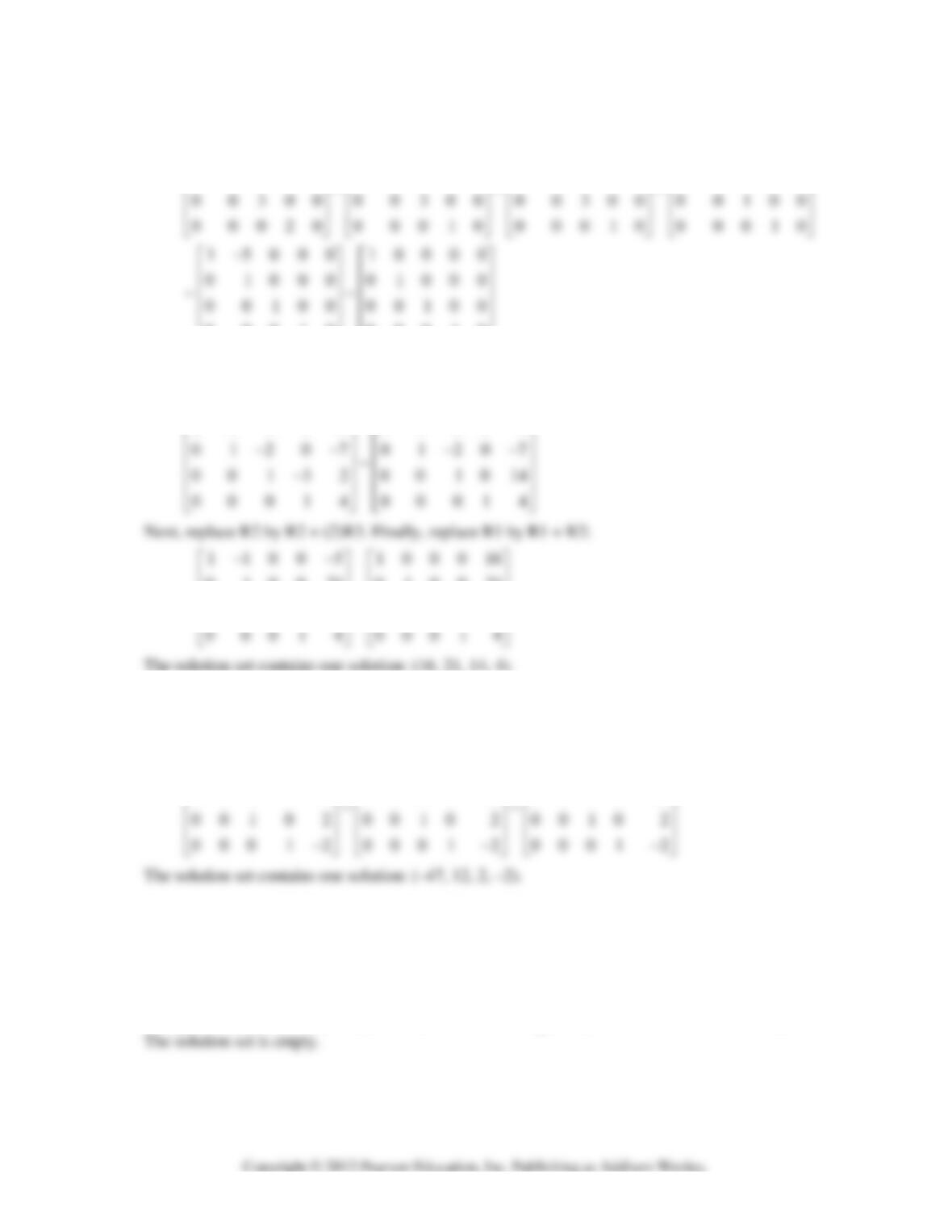
The solution set contains one solution: (0, 0, 0, 0).
9. The system has already been reduced to triangular form. Begin by replacing R3 by R3 + (3)R4:
11005 11005
−−−−
⎡⎤⎡⎤
010021 010021
~~
001014 001014
⎢⎥⎢⎥
⎢⎥⎢⎥
⎢⎥⎢⎥
10. The system has already been reduced to triangular form. Use the 1 in the fourth row to change the 3
and –2 above it to zeros. That is, replace R2 by R2 + (-3)R4 and replace R1 by R1 + (2)R4. For the
final step, replace R1 by R1 + (-3)R2.
130 2 7 1300 11 1000 47
010 3 6 0100 12 0100 12
−− − −
⎡⎤⎡⎤⎡⎤
⎢⎥⎢⎥⎢⎥
11. First, swap R1 and R2. Then replace R3 by R3 + (–2)R1. Finally, replace R3 by R3 + (1)R2.
0154 1432 1432 1432
143 2~0 15 4~0 1 5 4~0 15 4
2712 2712 0152 0002
−− −−
⎡⎤⎡⎤⎡ ⎤⎡⎤
⎢⎥⎢⎥⎢ ⎥⎢⎥
−− −−
⎢⎥⎢⎥⎢ ⎥⎢⎥
⎢⎥⎢⎥⎢ ⎥⎢⎥
−−−− −
⎣⎦⎣⎦⎣ ⎦⎣⎦
The system is inconsistent, because the last row would require that 0 = –2 if there were a solution.
4 CHAPTER 1 • Linear Equations in Linear Algebra
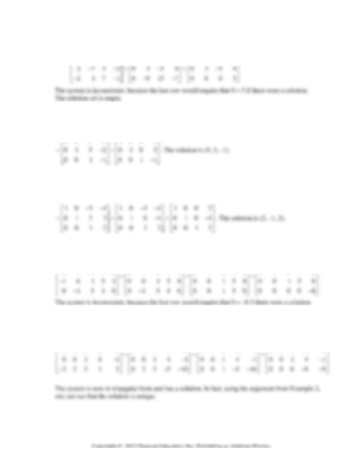
12. Replace R2 by R2 + (–2)R1 and replace R3 by R3 + (2)R1. Finally, replace R3 by R3 + (3)R2.
1543 1543 1543
−− − − − −
⎡⎤⎡⎤⎡⎤
13.
10 3 8 10 3 8 10 3 8 10 3 8
2297~02159~0152~0152
01 5 2 01 5 2 0215 9 00 5 5
−−−−
⎡⎤⎡⎤⎡⎤⎡⎤
⎢⎥⎢⎥⎢⎥⎢⎥
−−−
⎢⎥⎢⎥⎢⎥⎢⎥
⎢⎥⎢⎥⎢⎥⎢⎥
−−−−
⎣⎦⎣⎦⎣⎦⎣⎦
10 3 8 100 5
−
14.
20 6 8 10 3 4 10 3 4 10 3 4
0123~0123~0123~012 3
3624 3624 0678 00510
−− −− −− − −
⎡⎤⎡⎤⎡⎤⎡ ⎤
⎢⎥⎢⎥⎢⎥⎢ ⎥
⎢⎥⎢⎥⎢⎥⎢ ⎥
⎢⎥⎢⎥⎢⎥⎢ ⎥
−− −− −−
⎣⎦⎣⎦⎣⎦⎣ ⎦
15. First, replace R3 by R3 + (1)R1, then replace R4 by R4 + (1)R2, and finally replace R4 by R4 + (–
1)R3.
1 6 005 1 6 005 1 6 005 1 6 00 5
01410 01410 01410 01410
−−−−
⎡⎤⎡⎤⎡⎤⎡⎤
⎢⎥⎢⎥⎢⎥⎢⎥
−−−−
16. First replace R4 by R4 + (3/2)R1 and replace R4 by R4 + (–2/3)R2. (One could also scale R1 and R2
before adding to R4, but the arithmetic is rather easy keeping R1 and R2 unchanged.) Finally, replace
R4 by R4 + (–1)R3.
200410 200410 200410 200410
0330 0 0330 0 0330 0 0330 0
−− −− −− −−
⎡ ⎤⎡⎤⎡⎤⎡⎤
⎢ ⎥⎢⎥⎢⎥⎢⎥
17. Row reduce the augmented matrix corresponding to the given system of three equations:
231 231 231
−−−
⎡⎤⎡⎤⎡⎤
18. Row reduce the augmented matrix corresponding to the given system of three equations:
24 4 4 2 4 4 4 24 4 4
⎡⎤⎡ ⎤⎡⎤
141 4
hh
⎡⎤⎡ ⎤
151 5
hh
−−
⎡⎤⎡ ⎤
21.
14 2 1 4 2
~
−−
⎡⎤⎡ ⎤
Write c for
12h−
. Then the second equation cx
= 0 has a solution
22.
412
412 ~
263 003
2
h
h
h
−
⎡⎤
−
⎡⎤
⎢⎥
⎢⎥
⎢⎥
−− −+
⎣⎦
⎣⎦
The system is consistent if and only if
32
h
−+
= 0, that is, if
23. a. True. See the remarks following the box titled Elementary Row Operations.
b. False. A 5 × 6 matrix has five rows.
24. a. False. The definition of row equivalent requires that there exist a sequence of row operations that
transforms one matrix into the other.
6 CHAPTER 1 • Linear Equations in Linear Algebra
25.
147 147 147
035 ~035 ~035
gg g
hh h
−− −
⎡⎤⎡ ⎤⎡ ⎤
⎢⎥⎢ ⎥⎢ ⎥
−− −
⎢⎥⎢ ⎥⎢ ⎥
26. Row reduce the augmented matrix for the given system:
2 4 1 2 /2 1 2 /2
ff f
⎡⎤⎡ ⎤⎡ ⎤
27. Row reduce the augmented matrix for the given system. Scale the first row by 1/a, which is possible
since a is nonzero. Then replace R2 by R2 + (–c)R1.
1/ / 1 / /
abf bafa ba fa
⎡⎤⎡ ⎤⎡ ⎤
28. A basic principle of this section is that row operations do not affect the solution set of a linear
system. Begin with a simple augmented matrix for which the solution is obviously (3, –2, –1), and
then perform any elementary row operations to produce other augmented matrices. Here are three
examples. The fact that they are all row equivalent proves that they all have the solution set (3, –2, –
1).
100 3 100 3 100 3
⎡⎤⎡⎤⎡⎤
29. Swap R1 and R3; swap R1 and R3.
30. Multiply R3 by –1/5; multiply R3 by –5.
33. The first equation was given. The others are:
21 3 213
(2040)/4,or4 60TT T TTT= +++ −−=
1.1 • Solutions 7
Rearranging,
12 4
430
460
TT T
TTT
−−=
−+ − =
34. Begin by interchanging R1 and R4, then create zeros in the first column:
410130 101440 101440
14 1060 141060 04 0 420
−− −− −−
⎡⎤⎡⎤⎡ ⎤
⎢⎥⎢⎥⎢ ⎥
−− −− −
⎢⎥⎢⎥⎢ ⎥
0 1 4 15 190 0 0 4 14 195 0 0 0 12 270
⎢⎥⎢⎥⎢⎥
−− −
⎣⎦⎣⎦⎣⎦
Scale R4 by 1/12, use R4 to create zeros in column 4, and then scale R3 by 1/4:
10 1 4 40 10 10 50 10 10 50
−−
⎡⎤⎡⎤⎡⎤
0 1 0 0 27.5
~.
001030.0
0 0 0 1 22.5
⎢⎥
⎢⎥
⎢⎥
⎣⎦
The solution is (20, 27.5, 30, 22.5).
Notes:
The Study Guide includes a “Mathematical Note” about statements, “If … , then … .”
This early in the course, students typically use single row operations to reduce a matrix. As a result,
even the small grid for Exercise 34 leads to about 80 multiplications or additions (not counting operations
with zero). This exercise should give students an appreciation for matrix programs such as MATLAB.
Exercise 14 in Section 1.10 returns to this problem and states the solution in case students have not
already solved the system of equations. Exercise 31 in Section 2.5 uses this same type of problem in
1.1 describes how to access the data that is available for all numerical exercises in the text. This feature
has the ability to save students time if they regularly have their matrix program at hand when studying
linear algebra. The MATLAB box also explains the basic commands replace, swap, and scale.
These commands are included in the text data sets, available from the text web site,
1.2 SOLUTIONS
Notes:
The key exercises are 1–20 and 23–28. (Students should work at least four or five from Exercises
7–14, in preparation for Section 1.5.)
2. Reduced echelon form: a. Echelon form: b and d. Not echelon: c.
3.
246 8~00 2 8~00 1 4
36912 00 3 12 00 3 12
−−
⎢⎥⎢ ⎥⎢ ⎥
⎢⎥⎢ ⎥⎢ ⎥
−− −−
⎣⎦⎣ ⎦⎣ ⎦
⎢
⎢
⎢
⎣
124 8 120 8
−
⎡⎤⎡ ⎤
124 8
⎡
⎤
4.
1245124512451245
2 4 5 4 ~ 0 0 3 6 ~ 0 3 12 18 ~ 0 1 4 6
4 5 4 2 0 3 12 18 0 0 3 6 0 0 3 6
⎡⎤⎡ ⎤⎡ ⎤⎡ ⎤
⎢⎥⎢ ⎥⎢ ⎥⎢ ⎥
−− −− −
⎢⎥⎢ ⎥⎢ ⎥⎢ ⎥
⎢⎥⎢ ⎥⎢ ⎥⎢ ⎥
−− − − − −−
⎣⎦⎣ ⎦⎣ ⎦⎣ ⎦
5. **0
,,
00000
⎡ ⎤⎡⎤⎡⎤
⎢ ⎥⎢⎥⎢⎥
⎣ ⎦⎣⎦⎣⎦
6.
**0
0,00,00
00 0000
⎡
⎤⎡ ⎤⎡ ⎤
⎢
⎥⎢ ⎥⎢ ⎥
⎢
⎥⎢ ⎥⎢ ⎥
⎢
⎥⎢ ⎥⎢ ⎥
⎣
⎦⎣ ⎦⎣ ⎦
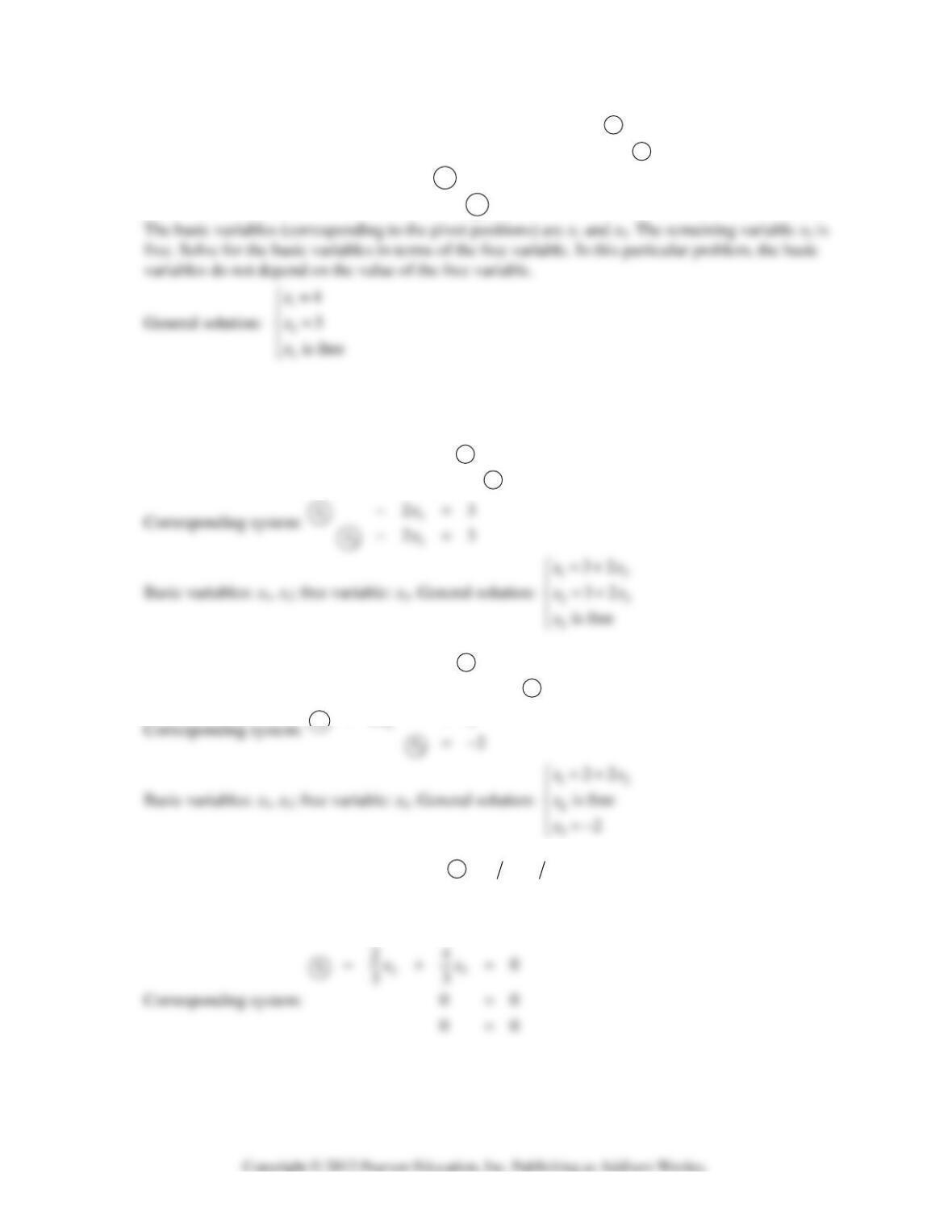
Corresponding system of equations:
12
3
35
3
xx
x
+=−
=
1.2 • Solutions 9
8. 1 305 1305 1305 1004
~~~
3 709 0206 0103 0103
−− −− −−
⎡⎤⎡⎤⎡⎤⎡⎤
⎢⎥⎢⎥⎢⎥⎢⎥
−−−
⎣⎦⎣⎦⎣⎦⎣⎦
Corresponding system of equations:
1
2
4
3
x
x
=
=
Note:
A common error in Exercise 8 is to assume that x
3
is zero. To avoid this, identify the basic
variables first. Any remaining variables are free. (This type of computation will arise in Chapter 5.)
9. 0123 1346 1023
~~
1346 0 12 3 0123
−−−−
⎡⎤⎡⎤⎡⎤
⎢⎥⎢⎥⎢⎥
−− − −
⎣⎦⎣⎦⎣⎦
10. 12 14 12 14 1202
~~
2456 00714 0012
−− −− −
⎡⎤⎡⎤⎡⎤
⎢⎥⎢⎥⎢⎥
−− − −
⎣⎦⎣⎦⎣⎦
22
xx
−=
11.
3240 3240 123430
96120~0000~0 0 0 0
6480 0000 0 0 0 0
−− −
⎡⎤⎡ ⎤⎡ ⎤
⎢⎥⎢ ⎥⎢ ⎥
−
⎢⎥⎢ ⎥⎢ ⎥
⎢⎥⎢ ⎥⎢ ⎥
−
⎣⎦⎣ ⎦⎣ ⎦
10 CHAPTER 1 • Linear Equations in Linear Algebra
123
24
33
xx
x
⎧=−
⎪
12. Since the bottom row of the matrix is equivalent to the equation 0 = 1, the system has no solutions.
13.
1 3 0 1 0 2 1 300 92 1000 35
0 1 0 0 4 1 0 100 41 0100 41
~~
0 0 0 1 9 4 0 001 94 0001 94
−−− − −
⎡⎤⎡⎤⎡⎤
⎢⎥⎢⎥⎢⎥
−−−
⎢⎥⎢⎥⎢⎥
⎢⎥⎢⎥⎢⎥
15
25
53
14
xx
xx
=+
⎧
⎪=+
Note:
The Study Guide discusses the common mistake x
3
= 0.
10 5 0 83 10 5 003
01 4 1 06 01 4 106
−− −
⎡⎤⎡⎤
⎢⎥⎢⎥
−−
13
234
5
35
64
xx
xxx
=+
⎧
⎪=− +
⎩
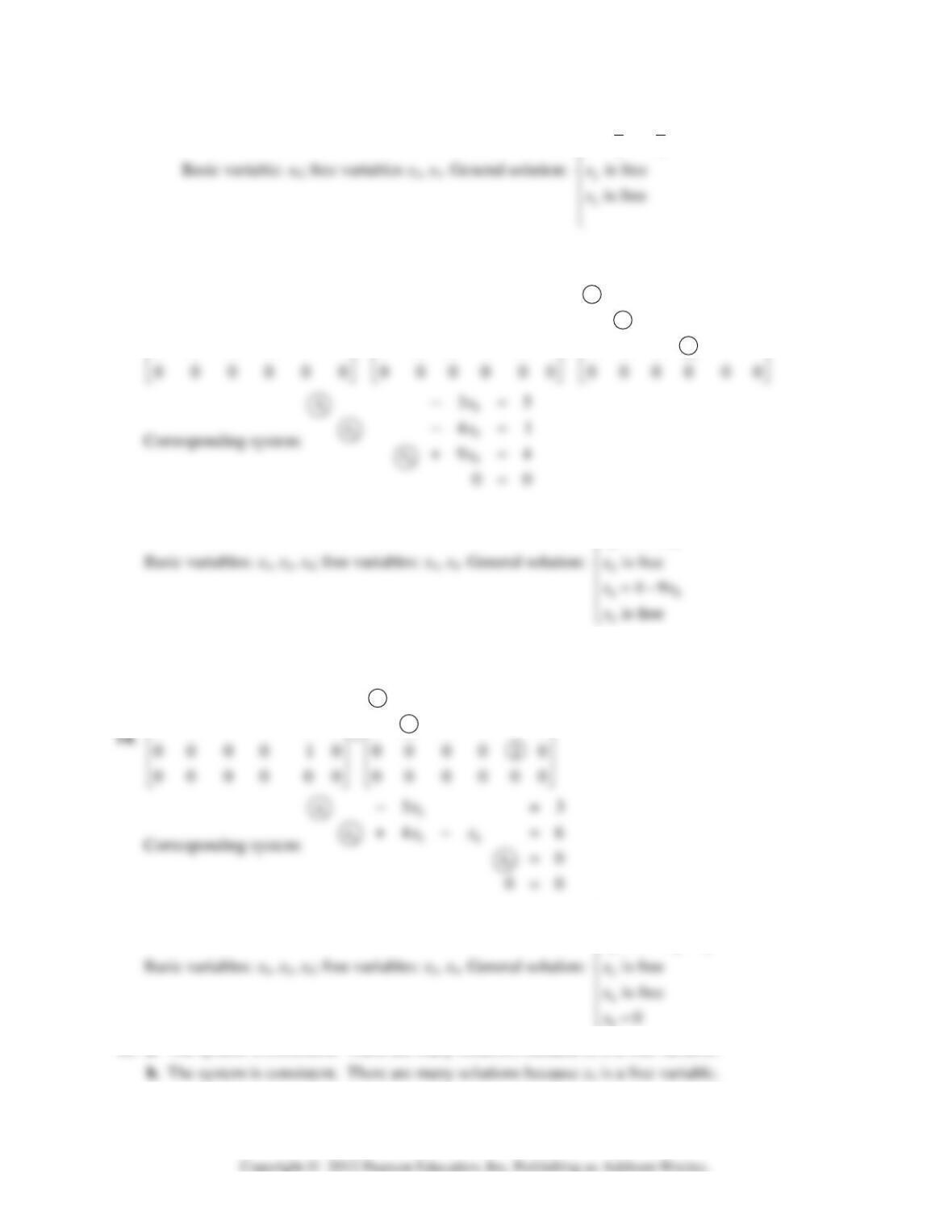
15. a. The system is consistent. There are many solutions because x
is a free variable.
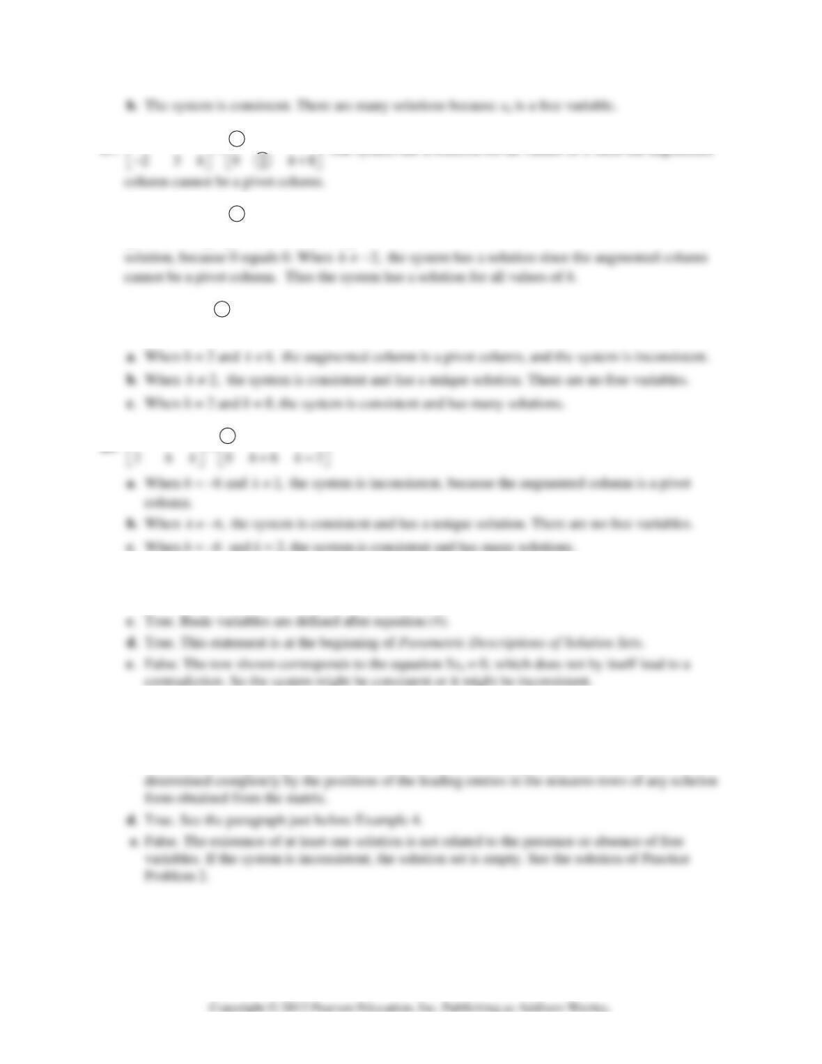
16. a. The system is inconsistent. (The rightmost column of the augmented matrix is a pivot column).
1.2 • Solutions 11
17. 114 11 4
−−
⎡⎤⎡ ⎤
The system has a solution for all values of h since the augmented
18. 13 1 1 3 1
~
62 036 2hhh
−−
⎡⎤⎡ ⎤
⎢⎥⎢ ⎥
−+−−
⎣⎦⎣ ⎦
If 3h + 6 is zero, that is, if h = –2, then the system has a
19.
121 2
~
48 084 8
hh
khk
⎡⎤⎡ ⎤
⎢⎥⎢ ⎥
−−
⎣⎦⎣ ⎦
20.
131 1 3 1
−−
⎡⎤⎡ ⎤
21. a. False. See Theorem 1.
b. False. See the second paragraph of the section.
22. a. True. See Theorem 1.
b. False. See Theorem 2.
c. False. See the beginning of the subsection Pivot Positions. The pivot positions in a matrix are
12 CHAPTER 1 • Linear Equations in Linear Algebra
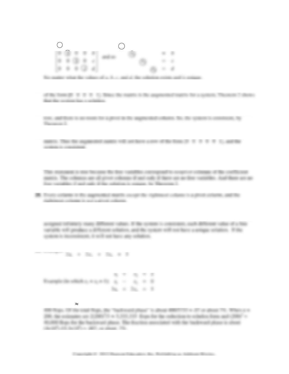
23. Since there are four pivots (one in each row), the augmented matrix must reduce to the form
1
1000
xa
a
=
⎡⎤
24. The system is consistent because there is not a pivot in column 5, which means that there is not a row
25. If the coefficient matrix has a pivot position in every row, then there is a pivot position in the bottom
26. Since the coefficient matrix has three pivot columns, there is a pivot in each row of the coefficient
27. “If a linear system is consistent, then the solution is unique if and only if every column in the
coefficient matrix is a pivot column; otherwise there are infinitely many solutions. ”
29. An underdetermined system always has more variables than equations. There cannot be more basic
variables than there are equations, so there must be at least one free variable. Such a variable may be
30. Example:
123
4
xx x
++=
31. Yes, a system of linear equations with more equations than unknowns can be consistent.
32. According to the numerical note in Section 1.2, when n = 20 the reduction to echelon form takes
about 2(20)
3
/3 5,333 flops, while further reduction to reduced echelon form needs at most (20)
2
=
1.2 • Solutions 13
33. For a quadratic polynomial p(t) = a
0
+ a
1
t + a
2
t
2
to exactly fit the data (1, 6), (2, 15), and (3, 28), the
coefficients a
0
, a
1
, a
2
must satisfy the systems of equations given in the text. Row reduce the
augmented matrix:
111 6 111 6 1116 1116
⎡⎤⎡⎤⎡⎤⎡⎤
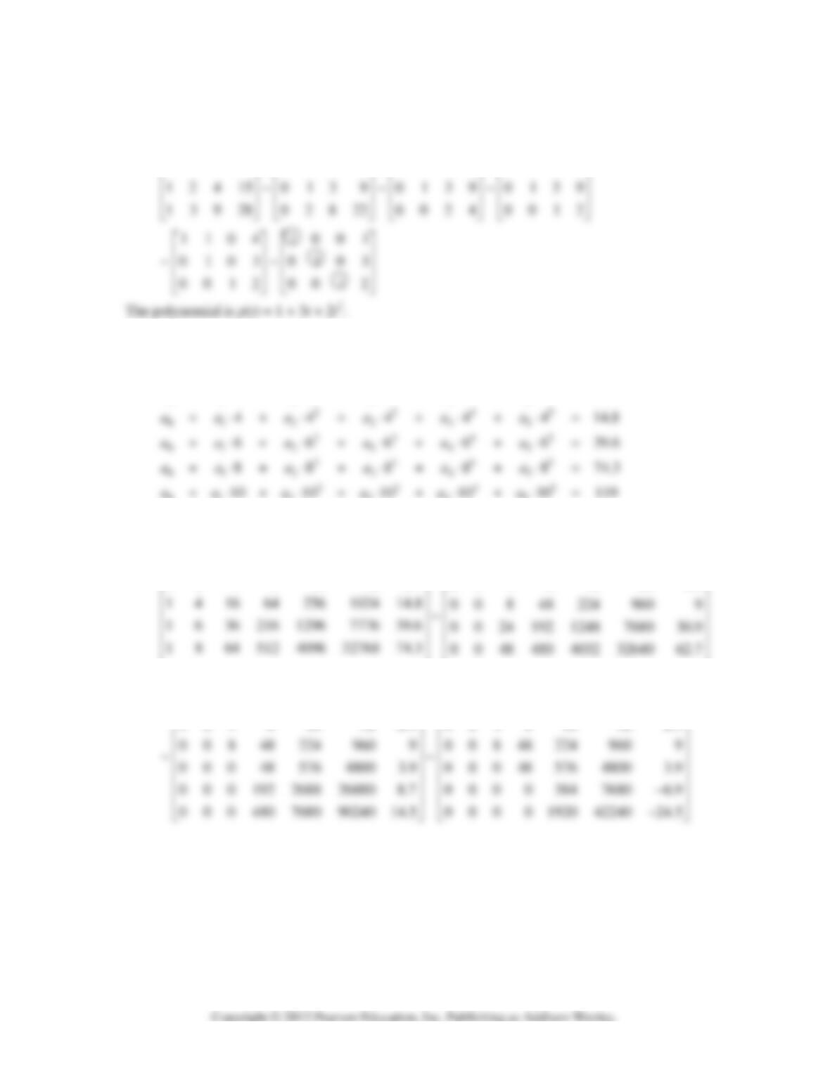
34. [M] The system of equations to be solved is:
2345
012345
2345
012345
01 2 3
000000
222222.90
aa a a a a
aaaaaa
+⋅+⋅+⋅+⋅+⋅=
+⋅+⋅+⋅+⋅+⋅=
45
The unknowns are a
0
, a
1
, …, a
5
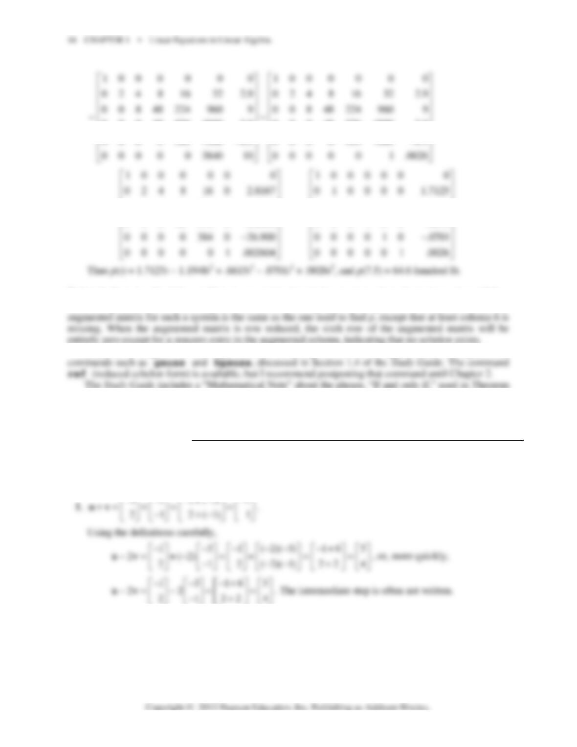
. Use technology to compute the reduced echelon of the augmented
matrix:
⎢
⎢
⎢
⎢
⎢
23 4 5
10 0 0 0 0 0 10 0 0 0 0 0
1 2 4 8 16 32 2.9 0 2 4 8 16 32 2.9
0 0 80 960 9920 99840 10
11010 10 10 10 119
⎡⎤
⎢⎥
⎢⎥
⎢⎥
⎣⎦4.5
⎡
⎤
⎢
⎥
⎢
⎥
⎢
⎥
⎣
⎦
100 0 0 0 0 100 0 0 0 0
0 2 4 8 16 32 2.9 0 2 4 8 16 32 2.9
⎡⎤⎡⎤
⎢⎥⎢⎥
000485764800 3.9 000485764800 3.9
⎢⎥⎢ ⎥
⎢⎥⎢ ⎥
0 0 8 48 224 0 6.5000 0 0 1 0 0 0 1.1948
~~~
000485760 8.6000 0 0 0 1 0 0 .6615
⎢⎥⎢⎥
⎢⎥⎢⎥
−
⎢⎥⎢⎥
−
“
Notes:
In Exercise 34, if the coefficients are retained to higher accuracy than shown here, then p(7.5) =
64.8. If a polynomial of lower degree is used, the resulting system of equations is overdetermined. The
Exercise 34 requires 25 row operations. It should give students an appreciation for higher-level
2.
1.3 SOLUTIONS
Notes:
The key exercises are 11–16, 19–22, 25, and 26. A discussion of Exercise 25 will help students
understand the notation [a
1
a
2
a
3
], {a
1
, a
2
, a
3
}, and Span{a
1
, a
2
, a
3
}.
1.3 • Solutions 15
2.
32325
+
⎡⎤ ⎡ ⎤ ⎡ ⎤ ⎡⎤
.
3. 4.
5.
12
352
203
898
xx
⎡⎤ ⎡⎤⎡⎤
⎢⎥ ⎢⎥⎢⎥
−+ =−
⎢⎥ ⎢⎥⎢⎥
⎢⎥ ⎢⎥⎢⎥
−
⎣⎦ ⎣⎦⎣⎦
,
12
1
12
35 2
203
89 8
xx
x
xx
⎡⎤⎡ ⎤⎡⎤
⎢⎥⎢ ⎥⎢⎥
−+ =−
⎢⎥⎢ ⎥⎢⎥
⎢⎥⎢ ⎥⎢⎥
−
⎣⎦⎣ ⎦⎣⎦
,
12
1
12
35 2
23
89 8
xx
x
xx
+
⎡
⎤⎡⎤
⎢
⎥⎢⎥
−=−
⎢
⎥⎢⎥
⎢
⎥⎢⎥
−
⎣
⎦⎣⎦
12
35 2
xx
+=
6.
123
37 20
23 10
xxx
−
⎡⎤ ⎡⎤ ⎡⎤⎡⎤
++ =
⎢⎥ ⎢⎥ ⎢⎥⎢⎥
−
⎣⎦ ⎣⎦ ⎣⎦⎣⎦
,
3
12
312
2
37 0
23 0
x
xx
xxx
−
⎡⎤⎡⎤⎡⎤
⎡
⎤
++ =
⎢⎥⎢⎥⎢⎥
⎢
⎥
−
⎣
⎦
⎣⎦⎣⎦⎣⎦ ,
123
123
37 2 0
23 0
xxx
xxx
+−
⎡⎤
⎡⎤
=
⎢⎥
⎢⎥
−+ + ⎣⎦
⎣⎦
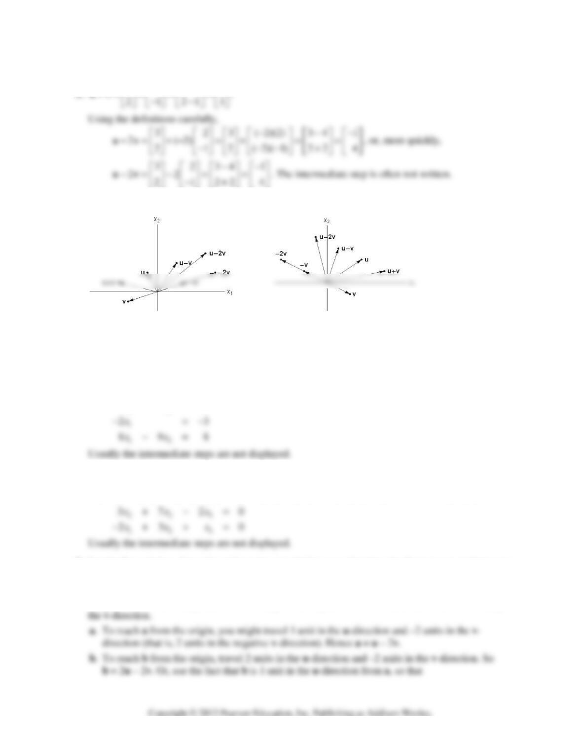
7. See the figure below. Since the grid can be extended in every direction, the figure suggests that every
vector in R
2
can be written as a linear combination of u and v.
To write a vector a as a linear combination of u and v, imagine walking from the origin to a along
the grid “streets” and keep track of how many “blocks” you travel in the u-direction and how many in
16 CHAPTER 1 • Linear Equations in Linear Algebra
b = a + u = (u – 2v) + u = 2u – 2v
Another solution is
d = b – 2v + u = (2u – 2v) – 2v + u = 3u – 4v
8. See the figure above. Since the grid can be extended in every direction, the figure suggests that every
vector in R
2
can be written as a linear combination of u and v.
w. To reach w from the origin, travel –1 units in the u–direction (that is, 1 unit in the negative
u-direction) and travel 2 units in the v-direction. Thus, w = (–1)u + 2v, or w = 2v – u.
x. To reach x from the origin, travel 2 units in the v–direction and –2 units in the u–direction. Thus,
x = –2u + 2v. Or, use the fact that x is –1 units in the u–direction from w, so that
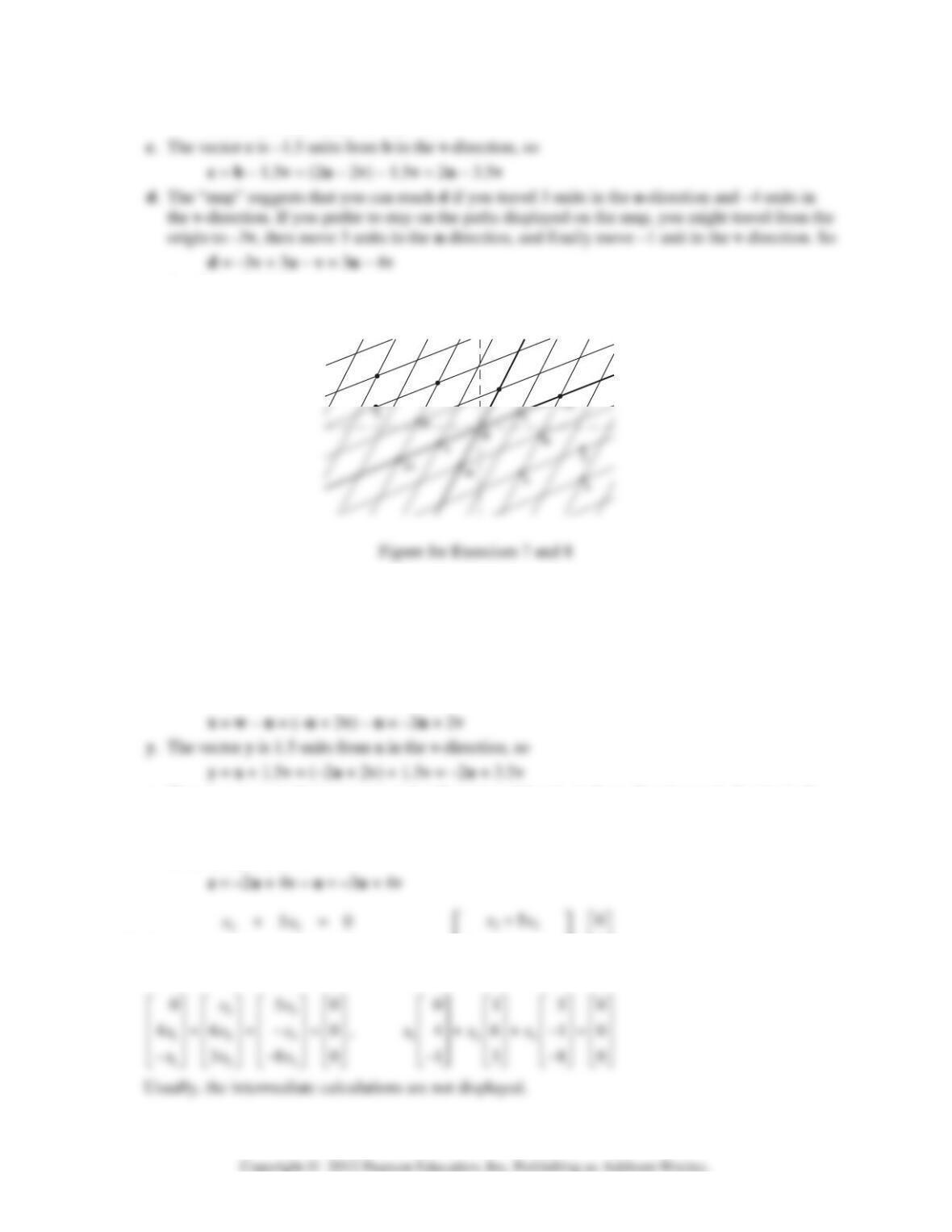
z. The map suggests that you can reach z if you travel 4 units in the v–direction and –3 units in the
u-direction. So z = 4v – 3u = –3u + 4v. If you prefer to stay on the paths displayed on the “map,”
you might travel from the origin to –2u, then 4 units in the v–direction, and finally move –1 unit
in the u–direction. So
⎡
9.
123
123
46 0
380
xxx
xxx
+−=
−+ − =
,
123
123
46 0
38 0
xxx
xxx
⎢⎥
⎢
⎥
+− =
⎢⎥
⎢
⎥
⎢⎥
⎢
⎥
−+ −
⎣
⎦
⎣⎦
u
d
b
1.3 • Solutions 17
Note:
The Study Guide says, “Check with your instructor whether you need to “show work” on a
problem such as Exercise 9.”
10.
123
123
123
32 4 3
27 5 1
54 32
xx x
xx x
xx x
−+=
−− + =
+−=
,
123
123
123
32 4 3
27 5 1
543 2
xx x
xxx
xxx
−+
⎡⎤
⎡
⎤
⎢⎥
⎢
⎥
−− + =
⎢⎥
⎢
⎥
⎢⎥
⎢
⎥
+−
⎣
⎦⎣⎦
⎡
⎢
⎢
⎢
⎣
11. The question
Is b a linear combination of a
1
, a
2
, and a
3
?
is equivalent to the question
Does the vector equation x
1
a
1
+ x
2
a
2
+ x
3
a
3
= b have a solution?
The equation
10 52
⎡⎤ ⎡⎤ ⎡⎤⎡⎤
has the same solution set as the linear system whose augmented matrix is
10 5 2
21 6 1
M
⎡⎤
⎢⎥
=− − −
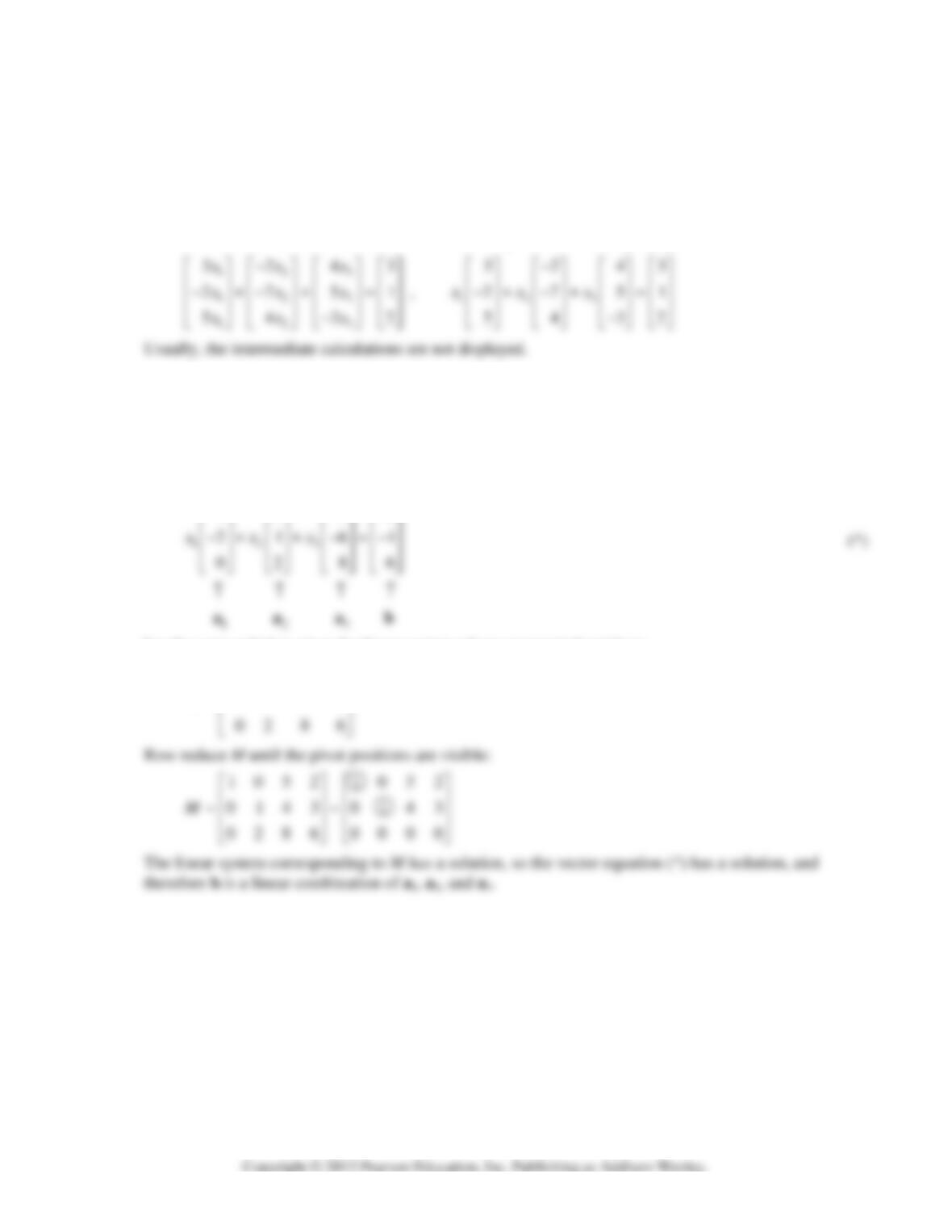
12. The equation
12 3
123
12611
0375
xx x
−−
⎡⎤ ⎡⎤ ⎡⎤⎡⎤
⎢⎥ ⎢⎥ ⎢⎥⎢⎥
++=−
⎢⎥ ⎢⎥ ⎢⎥⎢⎥
(*)
has the same solution set as the linear system whose augmented matrix is
12611
−−
⎡⎤
Row reduce M until the pivot positions are visible:
12611
−−
⎡⎤
13. Denote the columns of A by a
1
, a
2
, a
3
. To determine if b is a linear combination of these columns,
use the boxed fact in the subsection Linear Combinations. Row reduce the augmented matrix
[a
1
a
2
a
3
b] until you reach echelon form:
⎢
⎢
⎢
⎣
1423 1423
−−
⎡
⎤⎡ ⎤
14. Row reduce the augmented matrix [a
1
a
2
a
3
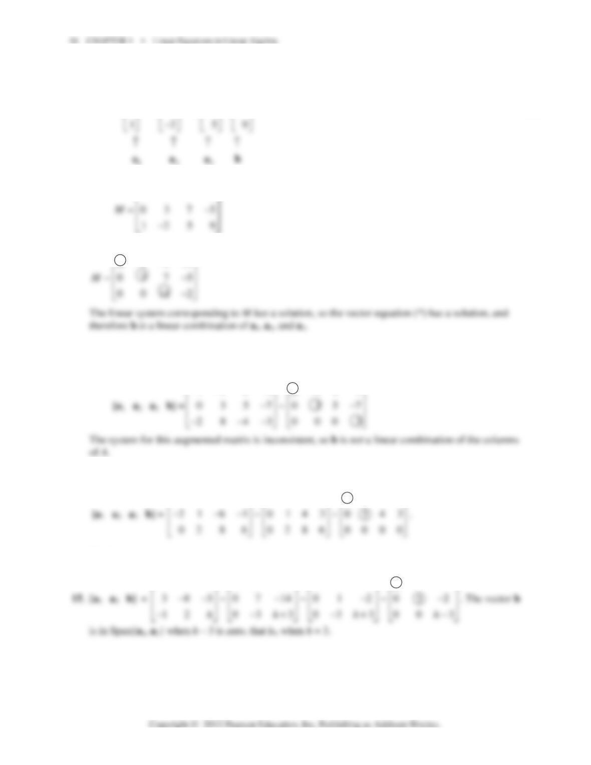
b] until you reach echelon form:
10 5 2 1052 1052
⎡⎤⎡⎤⎡⎤
The linear system corresponding to this matrix has a solution, so b is a linear combination of the
columns of A.
153 15 3 15 3 15 3
−−−−
⎡⎤⎡⎤⎡⎤⎡⎤
1.3 • Solutions 19
16. [v
1
v
2
y] =
12 12 12
013~01 3~01 3
hh h
−− −
⎡⎤⎡ ⎤⎡ ⎤
⎢⎥⎢ ⎥⎢ ⎥
−− −
. The vector y is in
17. Noninteger weights are acceptable, of course, but some simple choices are 0 v
1
+ 0 v
2
= 0, and
18. Some likely choices are 0 v
1
+ 0 v
2
= 0, and
1
2
−
1
−
3
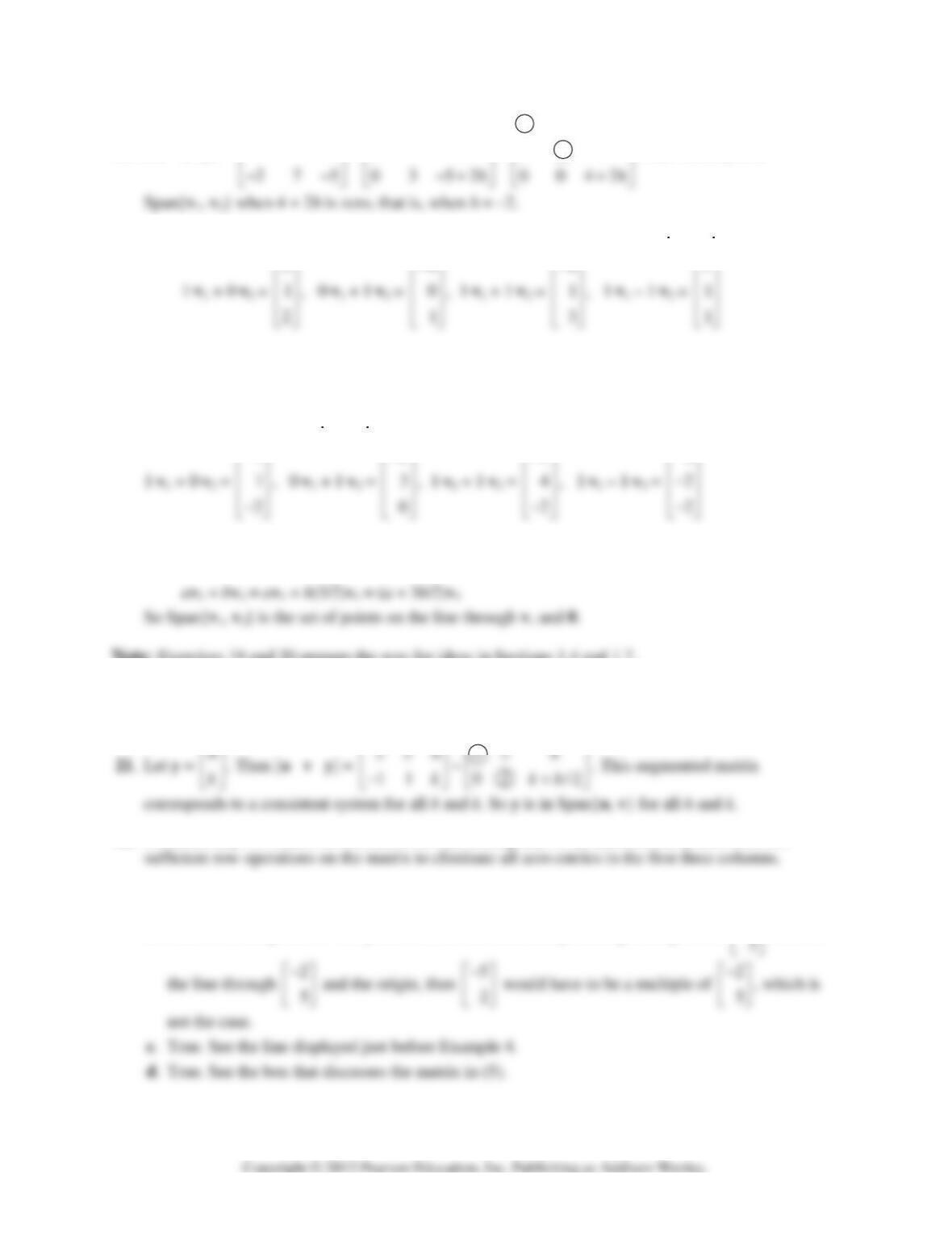
19. By inspection, v
2
= (3/2)v
1
. Any linear combination of v
1
and v
2
is actually just a multiple of v
1
. For
instance,
Note:
Exercises 19 and 20 prepare the way for ideas in Sections 1.4 and 1.7.
20. Span{v
1
, v
2
} is a plane in R
3
through the origin, because neither vector in this problem is a multiple
of the other.
22. Construct any 3×4 matrix in echelon form that corresponds to an inconsistent system. Perform
23. a. False. The alternative notation for a (column) vector is (–4, 3), using parentheses and commas.
b. False. Plot the points to verify this. Or, see the statement preceding Example 3. If
5
−
⎡⎤
⎢⎥
were on
24. a. False. Span{u, v} can be a plane.
b. True. See the beginning of the subsection Vectors in R
n
.
25. a. There are only three vectors in the set {a
1
, a
2
, a
3
}, and b is not one of them.
b. There are infinitely many vectors in W = Span{a
1
, a
2
, a
3
}. To determine if b is in W, use the
method of Exercise 13.
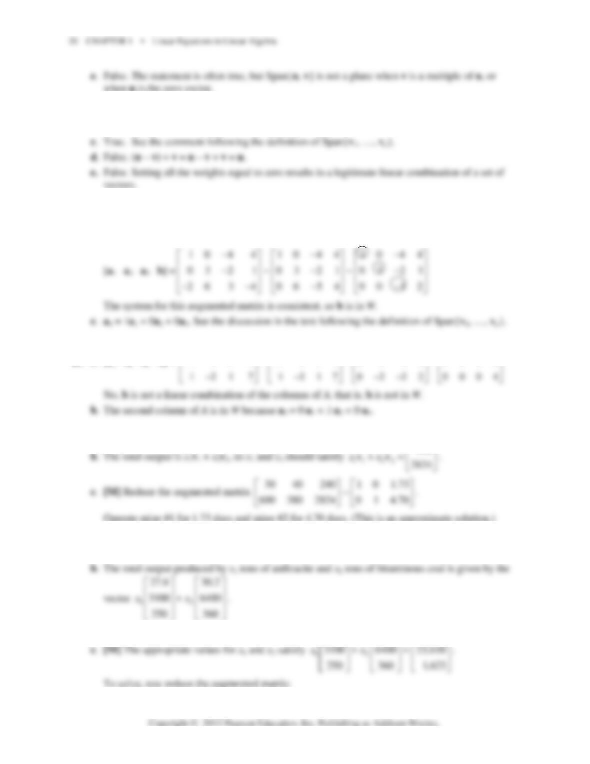
26. a. [a
⎢
⎢
⎣
a
a
b] =
2 0610 1 035 1 0 35 1035
1853~1853~0888~0888
−−
⎡
⎤⎡ ⎤⎡ ⎤⎡ ⎤
⎢
⎥⎢ ⎥⎢ ⎥⎢ ⎥
27. a. 5v
1
is the output of 5 days’ operation of mine #1.
⎢
⎣
⎡
⎢
⎣
240
⎡
⎤
28. a. The amount of heat produced when the steam plant burns x
1
tons of anthracite and x
2
tons of
bituminous coal is 27.6x
1
+ 30.2x
2
million Btu.
⎢
⎢
⎢
⎣
27.6 30.2 162
⎡
⎤⎡⎤⎡ ⎤