1.6 • Solutions 41
Move all variables to the left side and combine like terms:
⎢
⎢
⎢
⎣
.9 – .1 – .2 0
FM S
pp p
=
.9 .1 .2 0
−−
⎡
⎤
c. [M] You can obtain the reduced echelon form with a matrix program.
.9 .1 .2 0 1 0 .301 0 The number of decimal
.8 .9 .4 0 ~ 0 1 .712 0 places displayed is
−− −
⎡⎤⎡⎤
⎢⎥⎢⎥
−− −
⎢⎥⎢⎥
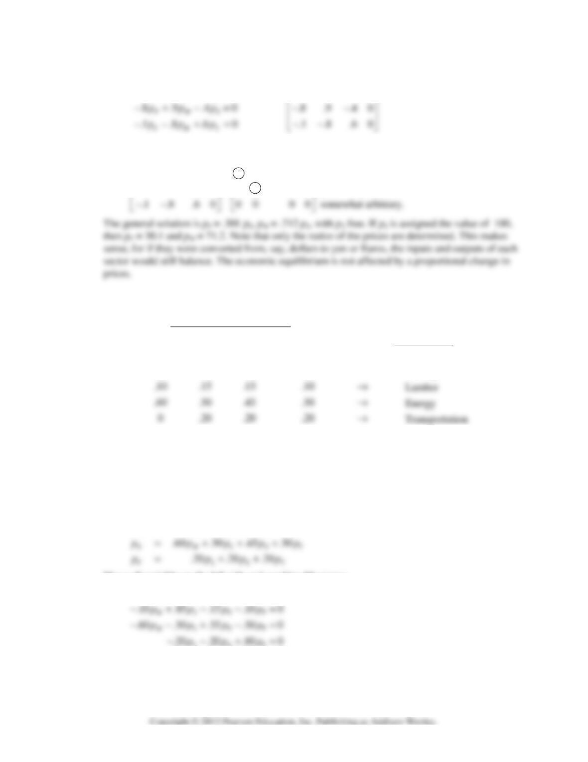
4. a. Fill in the exchange table one column at a time. The entries in each column must sum to 1.
Distribution of Output From :
Purchased by :
Mining Lumber Energy Transportation
output input
.30 .15 .20 .20 Mining
↓↓↓ ↓
→
b. [M] Denote the total annual output of the sectors by p
M
, p
L
, p
E
, and p
T
, respectively. From the first
row of the table, the total input to Agriculture is .30p
M
+ .15p
L
+ .20p
E
+ .20 p
T
. So the
equilibrium prices must satisfy
income expenses
.30 .15 .20 .20
MMLET
ppppp
=++ +
From the second, third, and fourth rows of the table, the equilibrium equations are
.10 .15 .15 .10
LMLET
ppppp
=+++
Move all variables to the left side and combine like terms:
.70 .15 .20 .20 0
MLET
LET
pppp
−−−=
Reduce the augmented matrix to reduced echelon form:
42 CHAPTER 1 • Linear Equations in Linear Algebra
.70 .15 .20 .20 0 1 0 0 1.37 0
−−− −
⎡⎤⎡⎤
Solve for the basic variables in terms of the free variable p
T
, and obtain p
M
= 1.37p
T
, p
L
= .84p
T
,
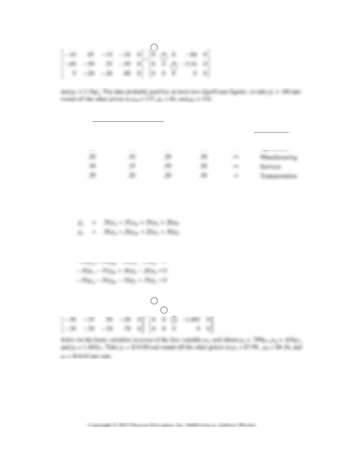
5. a. Fill in the exchange table one column at a time. The entries in each column must sum to 1.
Distribution of Output From :
Purchased by :
Agriculture Manufacturing Services Transportation
output input
.20 .35 .10 .20 Agriculture
↓↓↓↓
→
b. [M] Denote the total annual output of the sectors by p
A
, p
M
, p
S
, and p
T
, respectively. The
equilibrium equations are
.20 .35 .10 .20
.20 .10 .20 .30
A
AM ST
MAMST
ppppp
ppppp
=+++
=+++
Move all variables to the left side and combine like terms:
.80 .35 .10 .20 0
AM ST
pp pp
−−−=
Reduce the augmented matrix to reduced echelon form:
.80 .35 .10 .20 0 1 0 0 .799 0
.20 .90 .20 .30 0 0 1 0 .836 0
−−− −
⎡⎤⎡⎤
⎢⎥⎢⎥
−−− −
⎢⎥⎢⎥
c. Construct the new exchange table one column at a time. The entries in each column must sum to 1.
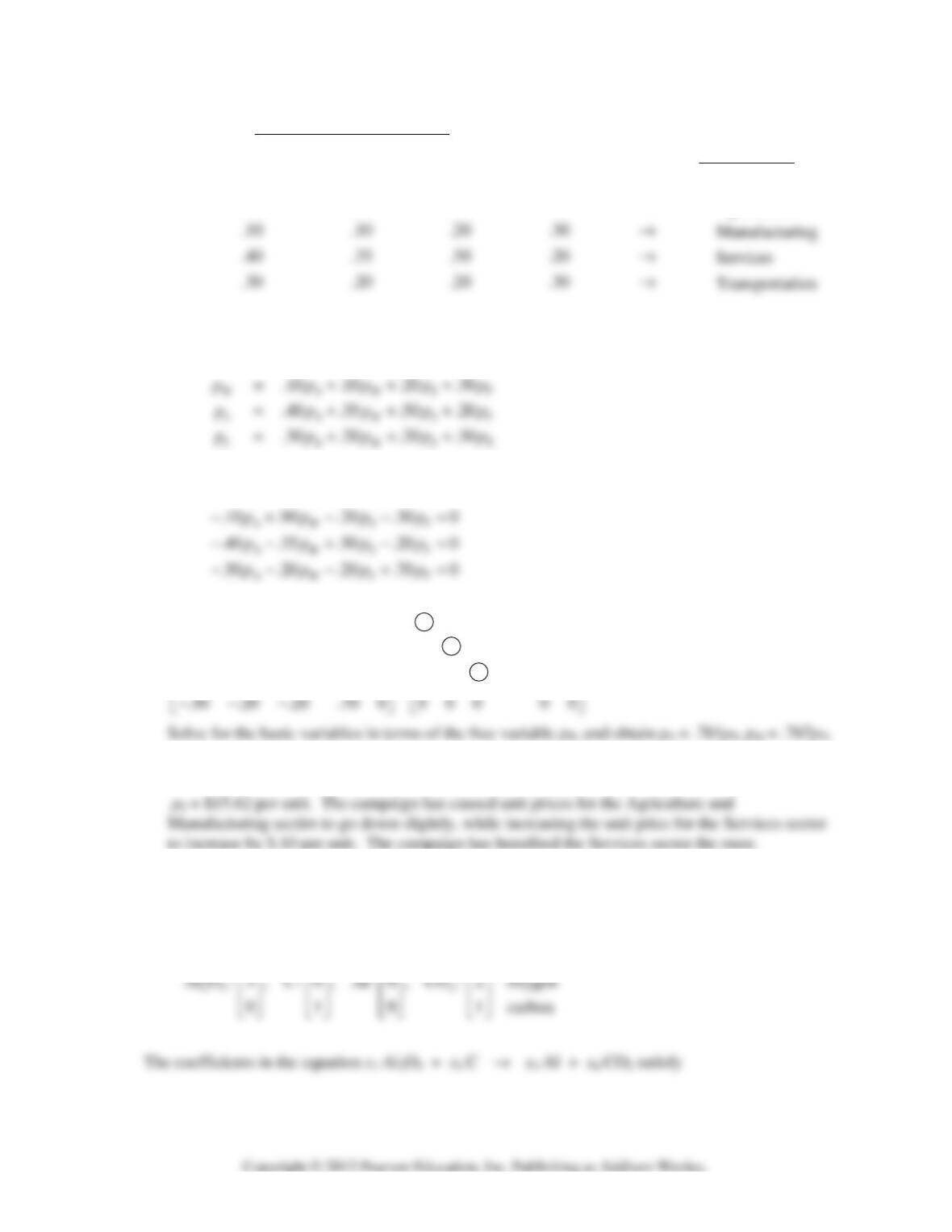
1.6 • Solutions 43
Distribution of Output From :
Purchased by :
Agriculture Manufacturing Services Transportation
output input
.20 .35 .10 .20 Agriculture
↓↓↓↓
→
d. [M] The new equilibrium equations are
.20 .35 .10 .20
A
AM ST
ppppp
=+++
Move all variables to the left side and combine like terms:
.80 .35 .10 .20 0
AM ST
pp pp
−−−=
Reduce the augmented matrix to reduced echelon form:
.80 .35 .10 .20 0 1 0 0 .781 0
.10 .90 .20 .30 0 0 1 0 .767 0
~
.40 .35 .50 .20 0 0 0 1 1.562 0
−−− −
⎡⎤⎡⎤
⎢⎥⎢⎥
−−− −
⎢⎥⎢⎥
⎢⎥⎢⎥
−− − −
⎢⎥⎢⎥
and
p
S
= 1.562p
T
. Take p
T
= $10.00 and round off the other prices to p
A
= $7.81, p
M
= $7.67, and
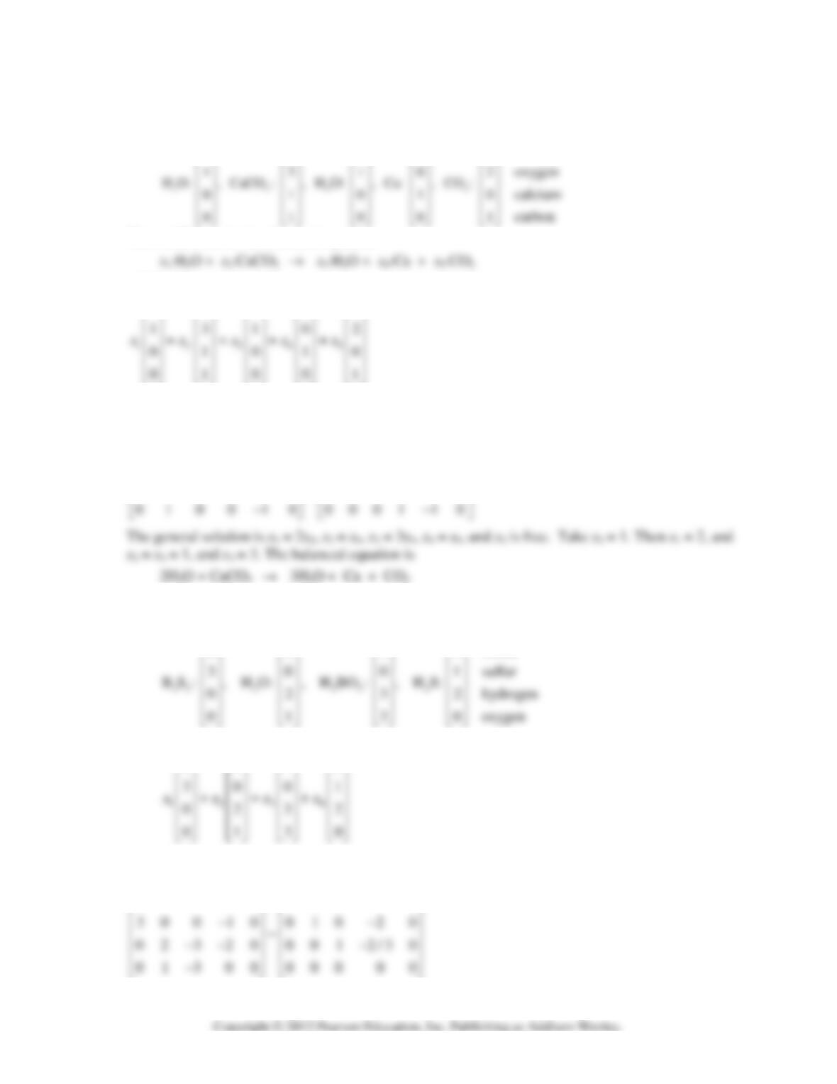
6. The following vectors list the numbers of atoms of aluminum (Al), oxygen (O), and carbon (C):
20 1 0
aluminum
⎡⎤ ⎡⎤ ⎡⎤ ⎡⎤
⎢⎥ ⎢⎥ ⎢⎥ ⎢⎥
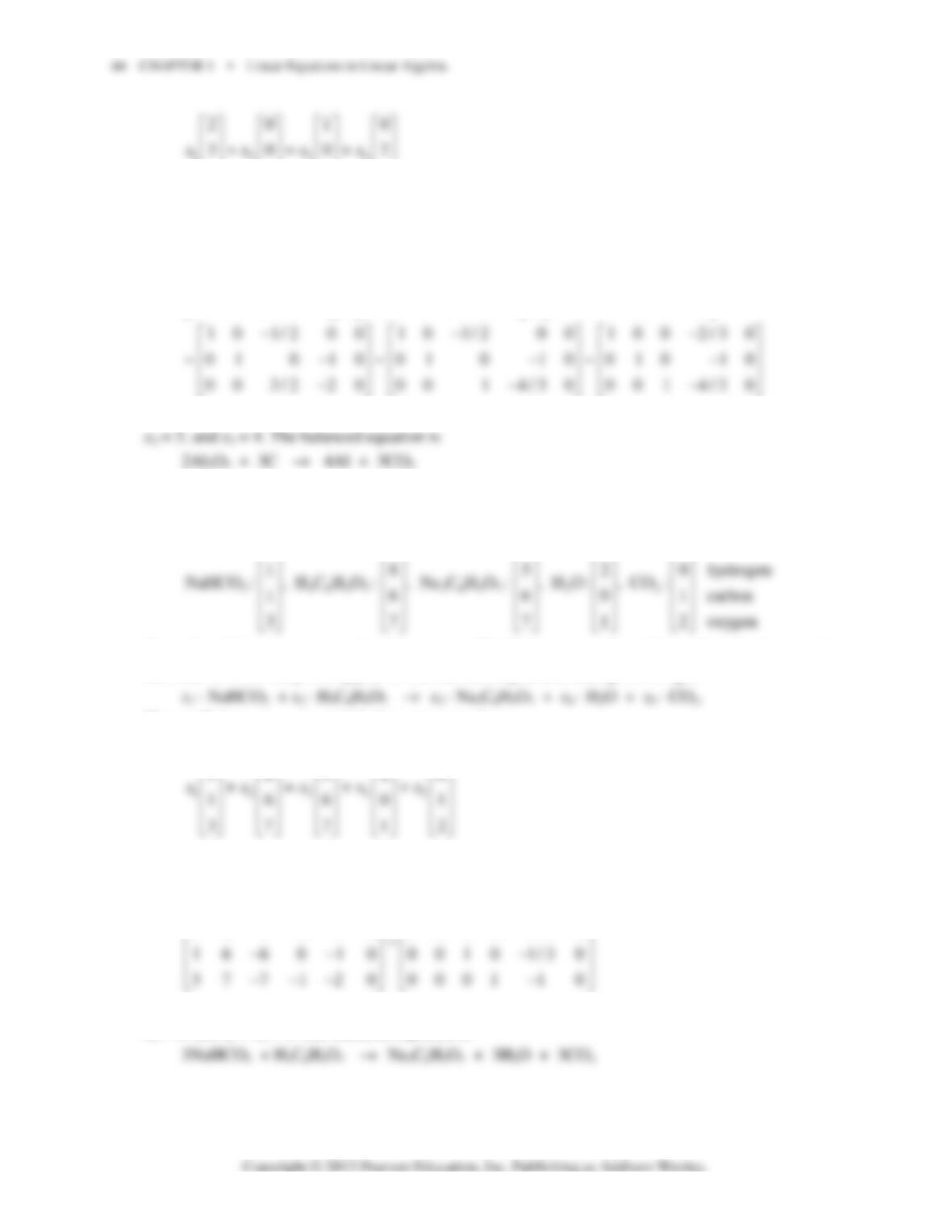
0101
⎢⎥ ⎢⎥ ⎢⎥ ⎢⎥
⎢⎥ ⎢⎥ ⎢⎥ ⎢⎥
⎣⎦ ⎣⎦ ⎣⎦ ⎣⎦
Move the right terms to the left side (changing the sign of each entry in the third and fourth vectors)
and row reduce the augmented matrix of the homogeneous system:
20 1 00 10 1/2 00 10 1/2 00
30 0 20~30 0 20~00 3/2 20
01 0 10 01 0 10 01 0 10
−− −
⎡⎤⎡⎤⎡⎤
⎢⎥⎢⎥⎢⎥
−−−
⎢⎥⎢⎥⎢⎥
⎢⎥⎢⎥⎢⎥
−−−
⎣⎦⎣⎦⎣⎦
The general solution is x
1
= (2/3)x
4
, x
2
= x
4
, x
3
= (4/3)x
4
, with x
4
free. Take x
4
= 3. Then x
1
= 2,
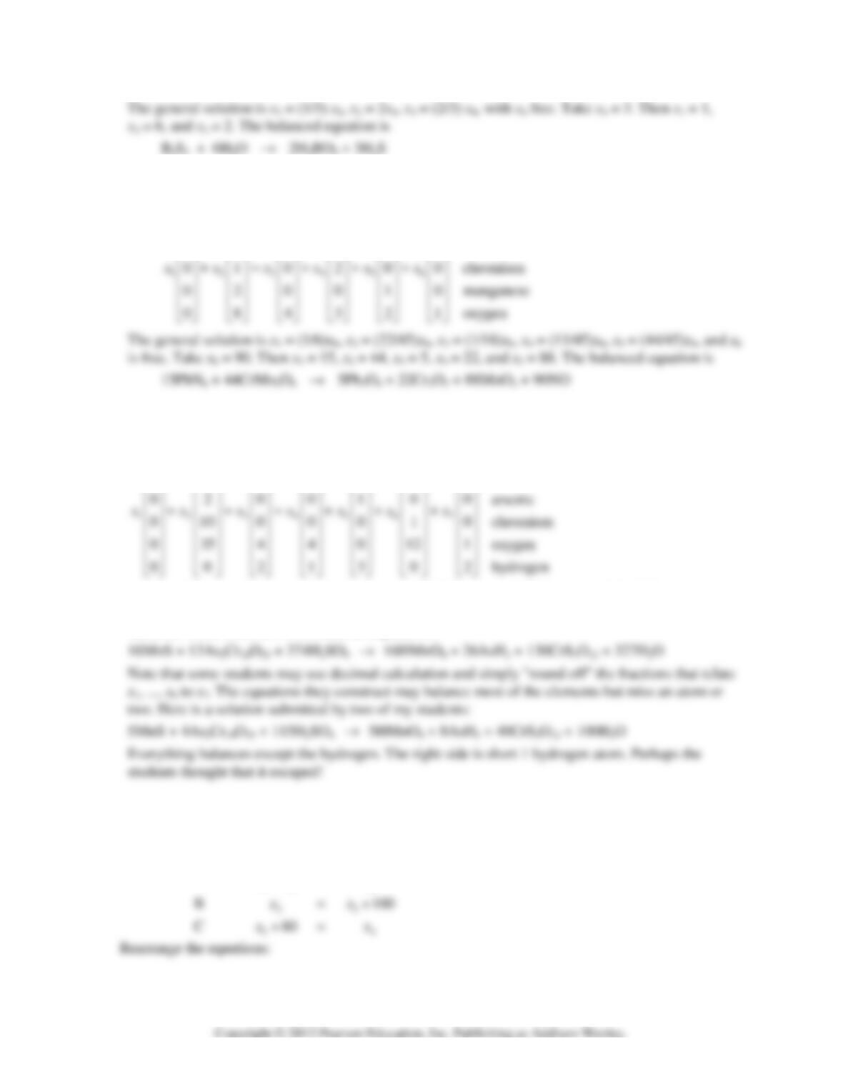
7. The following vectors list the numbers of atoms of sodium (Na), hydrogen (H), carbon (C), and
oxygen (O):
1 0 3 0 0 sodium
⎡⎤ ⎡⎤ ⎡⎤ ⎡⎤ ⎡⎤
The order of the various atoms is not important. The list here was selected by writing the elements in
the order in which they first appear in the chemical equation, reading left to right:
The coefficients x
1
, …, x
5
satisfy the vector equation
10300
⎡⎤ ⎡⎤ ⎡⎤ ⎡⎤ ⎡⎤
⎢⎥ ⎢⎥ ⎢⎥ ⎢⎥ ⎢⎥
Move all the terms to the left side (changing the sign of each entry in the third, fourth, and fifth
vectors) and reduce the augmented matrix:
1 0 3 0 0 0 1000 1 0
18 5 2 00 0100 1/30
−−
⎡⎤⎡⎤
⎢⎥⎢⎥
−− −
The general solution is x
1
= x
5
, x
2
= (1/3)x
5
, x
3
= (1/3)x
5
, x
4
= x
5
, and x
5
is free. Take x
5
= 3. Then x
1
=
x
4
= 3, and x
2
= x
3
= 1. The balanced equation is
1.6 • Solutions 45
8. The following vectors list the numbers of atoms of hydrogen (H), oxygen (O), calcium (Ca), and
carbon (C):
30200
hydrogen
⎡⎤ ⎡⎤ ⎡⎤ ⎡⎤ ⎡⎤
The coefficients in the chemical equation
satisfy the vector equation
30200
⎡⎤ ⎡⎤ ⎡⎤ ⎡⎤ ⎡⎤
Move the terms to the left side (changing the sign of each entry in the last three vectors) and reduce
the augmented matrix:
3 0 2 0 0 0 1000 2 0
1 3 1 0 2 0 0100 1 0
~
0 1 0 1 0 0 0010 30
−−
⎡⎤⎡⎤
⎢⎥⎢⎥
−− −
⎢⎥⎢⎥
⎢⎥⎢⎥
−−
9.The following vectors list the numbers of atoms of boron (B), sulfur (S), hydrogen (H), and oxygen
(O):
2 0 1 0 boron
⎡⎤ ⎡⎤ ⎡⎤ ⎡⎤
The coefficients in the equation x
1
⋅B
2
S
3
+ x
2
⋅H
2
O → x
3
⋅H
3
BO
3
+ x
4
⋅H
2
S satisfy
2010
⎡⎤ ⎡⎤ ⎡⎤ ⎡⎤
Move the terms to the left side (changing the sign of each entry in the third and fourth vectors) and
row reduce the augmented matrix of the homogeneous system:
20 1 00 100 1/30
−−
⎡⎤⎡ ⎤
46 CHAPTER 1 • Linear Equations in Linear Algebra
10. [M] Set up vectors that list the atoms per molecule. Using the order lead (Pb), nitrogen (N),
chromium (Cr), manganese (Mn), and oxygen (O), the vector equation to be solved is
103000lead
6 0 0 0 0 1 nitrogen
⎡⎤ ⎡⎤ ⎡⎤ ⎡⎤ ⎡⎤ ⎡⎤
⎢⎥ ⎢⎥ ⎢⎥ ⎢⎥ ⎢⎥ ⎢⎥
⎢⎥ ⎢⎥ ⎢⎥ ⎢⎥ ⎢⎥ ⎢⎥
11. [M] Set up vectors that list the atoms per molecule. Using the order manganese (Mn), sulfur (S),
arsenic (As), chromium (Cr), oxygen (O), and hydrogen (H), the vector equation to be solved is
1001000
1010030
⎡⎤ ⎡ ⎤ ⎡⎤ ⎡⎤ ⎡⎤ ⎡ ⎤ ⎡⎤
⎢⎥ ⎢ ⎥ ⎢⎥ ⎢⎥ ⎢⎥ ⎢ ⎥ ⎢⎥
⎢⎥ ⎢ ⎥ ⎢⎥ ⎢⎥ ⎢⎥ ⎢ ⎥ ⎢⎥
manganese
sulfur
In rational format, the general solution is x
1
= (16/327)x
7
, x
2
= (13/327)x
7
, x
3
= (374/327)x
7
,
x
4
= (16/327)x
7
, x
5
= (26/327)x
7
, x
6
= (130/327)x
7
, and x
7
is free. Take x
7
= 327 to make the other
variables whole numbers. The balanced equation is
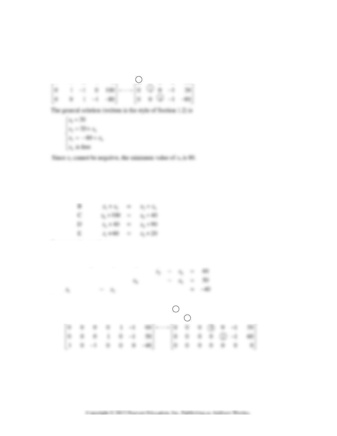
12. Write the equations for each intersection:
14 2
Intersection Flow in Flow out
A
xx x
+=
1.6 • Solutions 47
12 4
23
34
0
100
80
xx x
xx
xx
−+=
−=
−=−
Reduce the augmented matrix:
1 101 0 100020
−
⎡⎤⎡⎤
13. Write the equations for each intersection:
21
Intersection Flow in Flow out
A3080
xx
+=+
Rearrange the equations:
12
2345
50
0
xx
xxxx
−=−
−+− =
Reduce the augmented matrix:
11000050 10100040
011110 0 01100010
−−−−
⎡⎤⎡⎤
⎢⎥⎢⎥
−− −
⎢⎥⎢⎥
48 CHAPTER 1 • Linear Equations in Linear Algebra
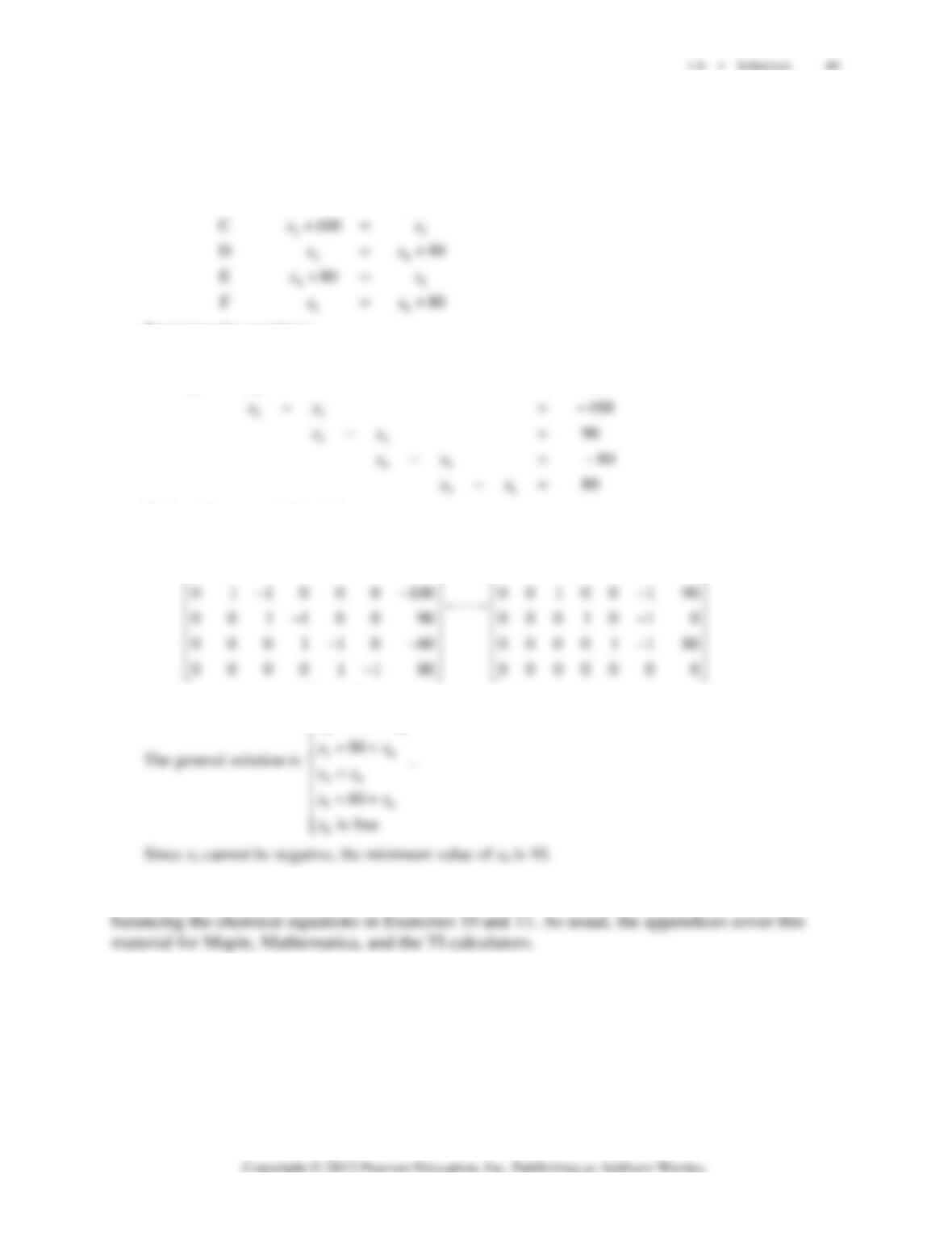
13
46
56
6
40
60
is free
xx
xx
x
=−
⎧
⎪
⎪
=+
⎪
⎪
⎩
b. To find minimum flows, note that since x
1
cannot be negative, x
3
> 40. This implies that
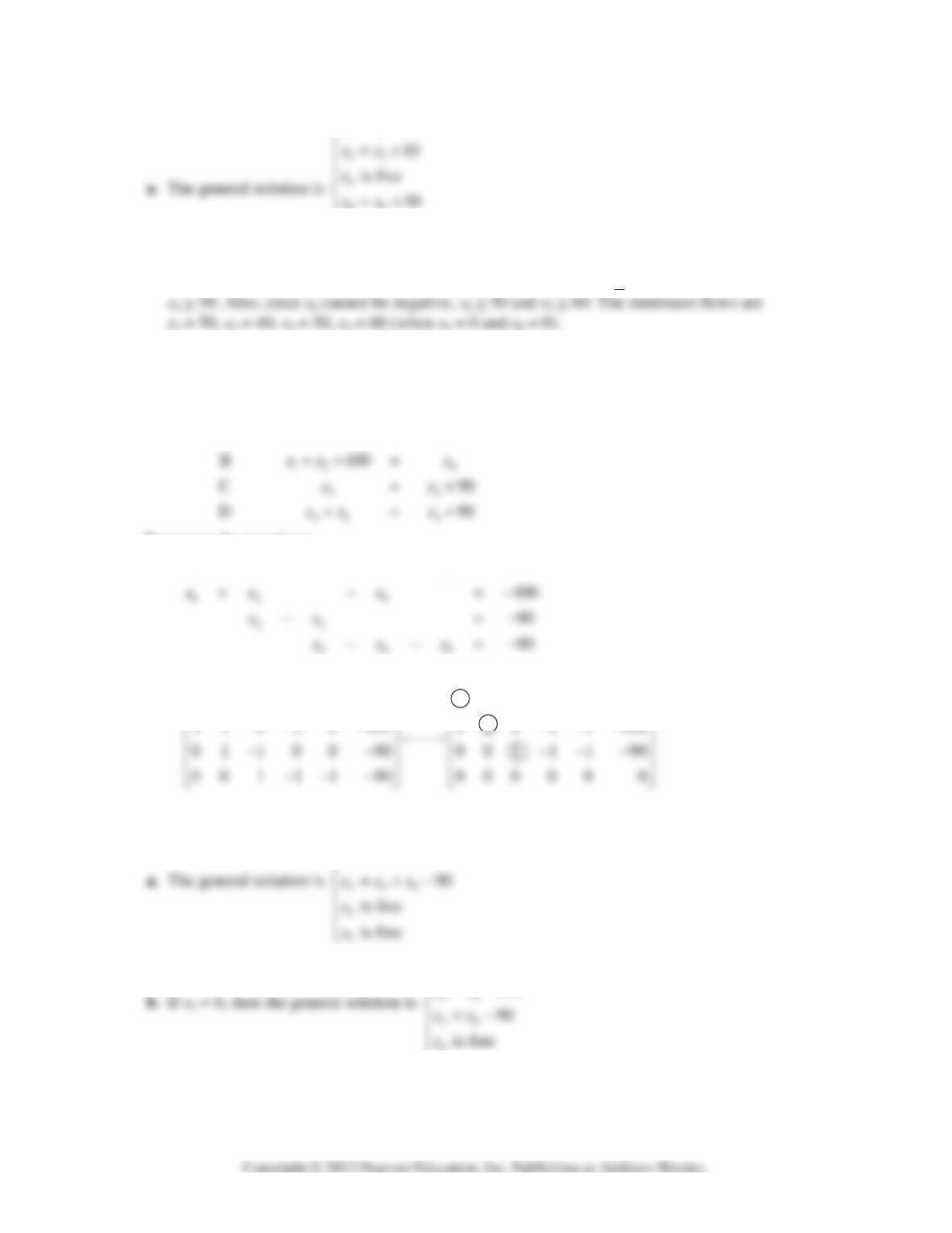
14. Write the equations for each intersection:
15
Intersection Flow in Flow out
A80
xx
=+
Rearrange the equations:
15
80
xx
+=
Reduce the augmented matrix:
10001 80 10001 80
⎡⎤⎡⎤
⎢⎥⎢⎥
15
245
80
180
xx
xxx
=−
⎧
⎪
=+−
⎪
1
4
80
180
x
xx
=
⎧
⎪
=−
⎩
c. Since x
2
cannot be negative, the minimum value of x
4
when x
5
= 0 is 180.
15. Write the equations for each intersection.
61
12
Intersection Flow in Flow out
A60
B70
xx
xx
+=
=+
Rearrange the equations:
16
12
60
70
xx
xx
−=
−=
Reduce the augmented matrix:
100001 60 10000160
110000 70 01000110
−−
⎡⎤⎡⎤
⎢⎥⎢⎥
−−−
⎢⎥⎢⎥
16
26
60
10
xx
xx
=+
⎧
⎪
=− +
Note: The MATLAB box in the Study Guide discusses rational calculations, needed for
1.7 SOLUTIONS
Note:
Key exercises are 9–20 and 23–30. Exercise 30 states a result that could be a theorem in the text.
There is a danger, however, that students will memorize the result without understanding the proof, and
then later mix up the words row and column. Exercises 37 and 38 anticipate the discussion in Section 1.9
of one-to-one transformations. Exercise 44 is fairly difficult for my students.
1. Use an augmented matrix to study the solution set of x
1
u + x
2
v + x
3
w = 0 (*), where u, v, and w are
5 7 90 5790
⎡⎤⎡⎤
2. Use an augmented matrix to study the solution set of x
1
u + x
2
v + x
3
w = 0 (*), where u, v, and w are
0010 20 30
−
⎡⎤⎡ ⎤
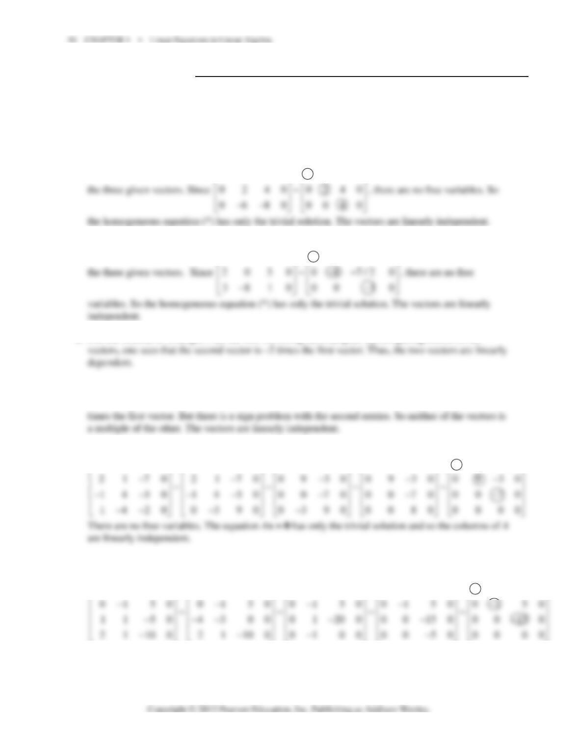
3. Use the method of Example 3 (or the box following the example). By comparing entries of the
4. From the first entries in the vectors, it seems that the second vector of the pair
13
,
39
−−
⎡⎤⎡⎤
⎢⎥⎢⎥
−
⎣⎦⎣⎦
may be 3
5. Use the method of Example 2. Row reduce the augmented matrix for Ax = 0:
0390 1420 1420 1420 1420
− −−−−−−−−
⎡ ⎤⎡ ⎤⎡⎤⎡⎤⎡⎤
6. Use the method of Example 2. Row reduce the augmented matrix for Ax = 0:
4 3 00 1 1 50 1 1 50 1 1 50 1 1 50
−− − − − −
⎡⎤⎡⎤⎡⎤⎡⎤⎡⎤
1.7 • Solutions 51
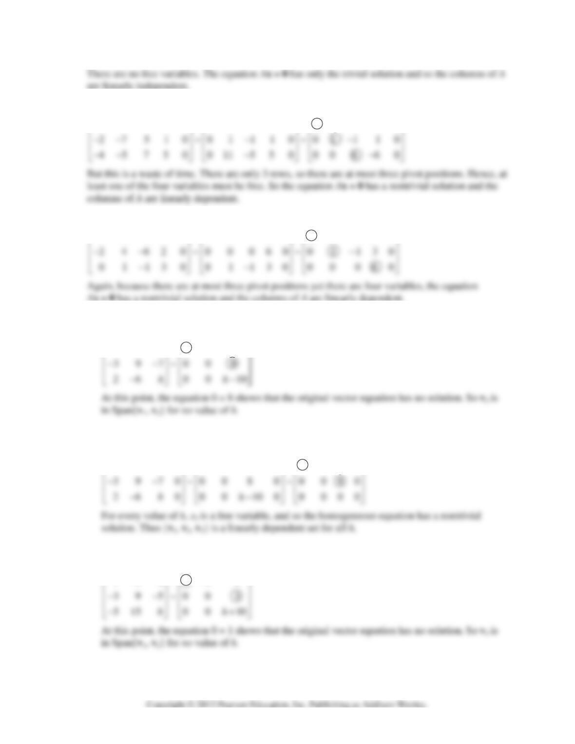
7. Study the equation Ax = 0. Some people may start with the method of Example 2:
14300 14300 14300
−−−
⎡⎤⎡⎤⎡⎤
8. Same situation as with Exercise 7. The (unnecessary) row operations are
12 320 12320 12 320
−−−
⎡⎤⎡⎤⎡⎤
Ax = 0 has a nontrivial solution and the columns of A are linearly dependent.
9. a. The vector v
3
is in Span{v
1
, v
2
} if and only if the equation x
1
v
1
+ x
2
v
2
= v
3
has a solution. To find
out, row reduce [v
1
v
2
v
3
], considered as an augmented matrix:
135 13 5
−−
⎡⎤⎡ ⎤
b. For {v
1
, v
2
, v
3
} to be linearly independent, the equation x
1
v
1
+ x
2
v
2
+ x
3
v
3
= 0 must have only the
trivial solution. Row reduce the augmented matrix [v
1
v
2
v
3
0]
1 3 50 1 3 5 0 1 350
−− −
⎡⎤⎡ ⎤⎡⎤
10. a. The vector v
3
is in Span{v
1
, v
2
} if and only if the equation x
1
v
1
+ x
2
v
2
= v
3
has a solution. To find
out, row reduce [v
1
v
2
v
3
], considered as an augmented matrix:
132 13 2
−−
⎡⎤⎡ ⎤
52 CHAPTER 1 • Linear Equations in Linear Algebra
b. For {v
1
, v
2
, v
3
} to be linearly independent, the equation x
1
v
1
+ x
2
v
2
+ x
3
v
3
= 0 must have only the
trivial solution. Row reduce the augmented matrix [v
1
v
2
v
3
0]
1320 13 2 0 1320
−− −
⎡⎤⎡ ⎤⎡⎤
11. To study the linear dependence of three vectors, say v
1
, v
2
, v
3
, row reduce the augmented matrix
[v
1
v
2
v
3
0]:
2420 24 20 24 20
−− −
⎡⎤⎡ ⎤⎡ ⎤
12. To study the linear dependence of three vectors, say v
1
, v
2
, v
3
, row reduce the augmented matrix
[v
1
v
2
v
3
0]:
18.
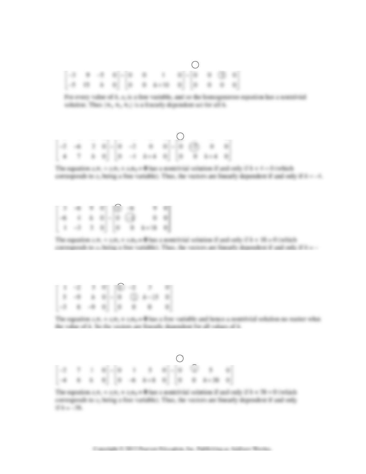
13. To study the linear dependence of three vectors, say v
1
, v
2
, v
3
, row reduce the augmented matrix
[v
1
v
2
v
3
0]:
14. To study the linear dependence of three vectors, say v
1
, v
2
, v
3
, row reduce the augmented matrix
[v
1
v
2
v
3
0]:
1320 13 20 13 2 0
−− −
⎡⎤⎡ ⎤⎡ ⎤
15. The set is linearly dependent, by Theorem 8, because there are four vectors in the set but only two
entries in each vector.
17. The set is linearly dependent, by Theorem 9, because the list of vectors contains a zero vector.
19. The set is linearly independent because neither vector is a multiple of the other vector. [Two of the
20. The set is linearly dependent, by Theorem 9, because the list of vectors contains a zero vector.
21. a. False. A homogeneous system always has the trivial solution. See the box before Example 2.
22. a. True. See Theorem 7.
b. True. See Example 4.
⎢
⎢
⎢
⎣
12
⎡
⎤⎡⎤
⎢
⎢
⎢
⎣
⎢
⎢
⎢
⎢
*0 00
**
⎡
⎤
*0
000
⎡
⎤⎡⎤
⎢
⎥⎢⎥
⎣
⎦⎣⎦
26.
**
0*
00
⎡⎤
⎢⎥
⎢⎥
⎢⎥
. The columns must be linearly independent, by Theorem 7, because the first column is
27. All four columns of the 6×4 matrix A must be pivot columns. Otherwise, the equation Ax = 0 would
28. If the columns of a 4×6 matrix A span R
4
, then A has a pivot in each row, by Theorem 4. Since each
29. A: any 3×2 matrix with one column a multiple of the other.
30. a. n
b. The columns of A are linearly independent if and only if the equation Ax = 0 has only the trivial
31. Think of A = [a
1
a
2
a
3
]. The text points out that a
3
= a
1
+ a
2
. Rewrite this as a
1
+ a
2
– a
3
= 0. As a
matrix equation, Ax = 0 for x = (1, 1, –1).
34. False. The vector v
1
could be the zero vector.
36. False. Counterexample: Take v
1
and v
2
to be multiples of one vector. Take v
3
to be not a multiple of
that vector. For example,
121
⎡⎤ ⎡ ⎤ ⎡ ⎤
37. True. A linear dependence relation among v
1
, v
2
, v
3
may be extended to a linear dependence relation
38. True. If the equation x
1
v
1
+ x
2
v
2
+ x
3
v
3
= 0 had a nontrivial solution (with at least one of x
1
, x
2
, x
3
39. If for all b the equation Ax = b has at most one solution, then take b = 0, and conclude that the
40. An m×n matrix with n pivot columns has a pivot in each column. So the equation Ax = b has no free
1.7 • Solutions 55
41. [M]
3 4 10 7 4 3 4 10 7 4
~
4 3 5 2 1 0 25/3 25/3 22/3 19/3
8 7 23 4 15 0 11/ 3 11/ 3 44 / 3 77 / 3
A
−−− −
⎡⎤⎡ ⎤
=
⎢⎥⎢ ⎥
−−
⎢⎥⎢ ⎥
−−−
⎣⎦⎣ ⎦
3410 7 43410 7 4
0 29/3 29/3 2/3 25/3 0 29/3 29/3 2/3 25/3
−−−−
⎡⎤⎡⎤
⎢⎥⎢⎥
−−
⎢
⎢
⎢
⎣
34 7
5311
−
⎡
⎤
⎢
⎥
−−−
42. [M]
121068414 1210 6 8 4 14
76457 9 0 1/61/21/314/35/6
~~
9999918 0 0 2 2 16 2
⎡
⎢
⎢
⎢
⎢
⎢
⎢
⎣
−− − −
⎡⎤⎡ ⎤
⎢⎥⎢ ⎥
−− −− − − −
⎢⎥⎢ ⎥
⎢⎥⎢ ⎥
⋅⋅⋅
−− −−−
43. [M] Make v any one of the columns of A that is not in B and row reduce the augmented matrix
44. [M] Calculations made as for Exercise 43 will show that each column of A that is not a column of B
is in the set spanned by the columns of B. Reason: The original matrix A has only four pivot
columns. If one or more columns of A are removed, the resulting matrix will have at most four pivot
columns. (Use exactly the same row operations on the new matrix that were used to reduce A to
56 CHAPTER 1 • Linear Equations in Linear Algebra
1.8 SOLUTIONS
Notes:
The key exercises are 17–20, 25 and 31. Exercise 20 is worth assigning even if you normally
assign only odd exercises. Exercise 25 (and 26) can be used to make a few comments about computer
Exercises 19 and 20 provide a natural segue into Section 1.9. I arrange to discuss the homework on
these exercises when I am ready to begin Section 1.9. The definition of the standard matrix in Section 1.9
to show that the coordinate mapping from a vector space onto R
n
(in Section 4.4) preserves linear
independence and dependence of sets of vectors. (See Example 6 in Section 4.4.)
1. T(u) = Au =
20 1 2
02 3 6
⎡⎤⎡⎤⎡⎤
=
⎢⎥⎢⎥⎢⎥
−−
⎣⎦⎣⎦⎣⎦
, T(v) =
20 2
02 2
aa
bb
⎡
⎤⎡ ⎤ ⎡ ⎤
=
⎢
⎥⎢ ⎥ ⎢ ⎥
⎣
⎦⎣ ⎦ ⎣ ⎦
3.
[]
1032 1032 1032
3163~0133~0133
2211 0253 0013
A
−− −− −−
⎡⎤⎡⎤⎡⎤
⎢⎥⎢⎥⎢⎥
=− − − − −
⎢⎥⎢⎥⎢⎥
⎢⎥⎢⎥⎢⎥
−−− − −−
⎣⎦⎣⎦⎣⎦
b
4.
[]
1236 1236 1236
0134~0134~0134
2565 0107 0033
A
−− −− −−
⎡⎤⎡⎤⎡⎤
⎢⎥⎢⎥⎢⎥
=−− −− −−
⎢⎥⎢⎥⎢⎥
⎢⎥⎢⎥⎢⎥
−− − −
⎣⎦⎣⎦⎣⎦
b
5.
[]
~~
37 52 0 12 1 0121
A−−− −−−
=
⎢⎥⎢⎥⎢⎥
−−
⎣⎦⎣⎦⎣⎦
b
Note that a solution is not
3
1
⎡⎤
⎢⎥
⎣⎦
. To avoid this common error, write the equations:
The general solution is
13
⎢
⎢
⎣
⎡
⎢
⎢
⎢
⎣
33 3 3
12 1 2
xx
xxx
−−
⎡⎤⎡ ⎤
⎡
⎤⎡⎤
⎢⎥⎢ ⎥
⎢
⎥⎢⎥
==−=+−
x
. For a particular solution, one might
1321 1321 1321 10810
3886 0123 0123 0123
−−−
⎡⎤⎡⎤⎡⎤⎡⎤
⎢⎥⎢⎥⎢⎥⎢⎥
−
3
⎩
⎢
⎢
⎢
⎣
⎡
⎢
⎢
⎢
⎣
13
10 8 10 8
xx
−−
⎡⎤⎡ ⎤
⎡
⎤⎡⎤
7. The value of a is 5. The domain of T is R
5
, because a 6×5 matrix has 5 columns and for Ax to be
5
1 3 5 50 1 3 5 50 1 3 5 50
−− −− −−
⎡⎤⎡⎤⎡⎤
58 CHAPTER 1 • Linear Equations in Linear Algebra
10 400
−
⎡⎤
13
40
xx
−=
13
4
xx
=
⎧
⎪
13
44
xx
⎡⎤⎡⎤ ⎡⎤
⎢⎥⎢⎥ ⎢⎥
10. Solve Ax = 0.
3210 60 10 2 40 102 40
10 2 40 3210 60 024 60
~~
−−−
⎡⎤⎡⎤⎡⎤
⎢⎥⎢⎥⎢⎥
−−
⎢⎥⎢⎥⎢⎥
⎢
⎢
⎢
⎣
240
xxx
+−=
134
24
23
xxx
xxx
=− +
⎧
⎪
=− −
⎪
4
3
4
224
3
223
x
x
x
xxx
−−
⎡⎤
⎡
⎤⎡⎤⎡⎤
⎢⎥
⎢
⎥⎢⎥⎢⎥
−
−−−
11. Is the system represented by [A b] consistent? Yes, as the following calculation shows.
13551 13551 13551
−−− −−− −−−
⎡⎤⎡⎤⎡⎤
12. Is the system represented by [A b] consistent?
321061 10243 1024 3
10 243 321061 024610
−− − −
⎡⎤⎡⎤⎡⎤
⎢⎥⎢⎥⎢⎥
−−−−
1.8 • Solutions 59
The system is inconsistent, so b is not in the range of the transformation
A
xx6
.
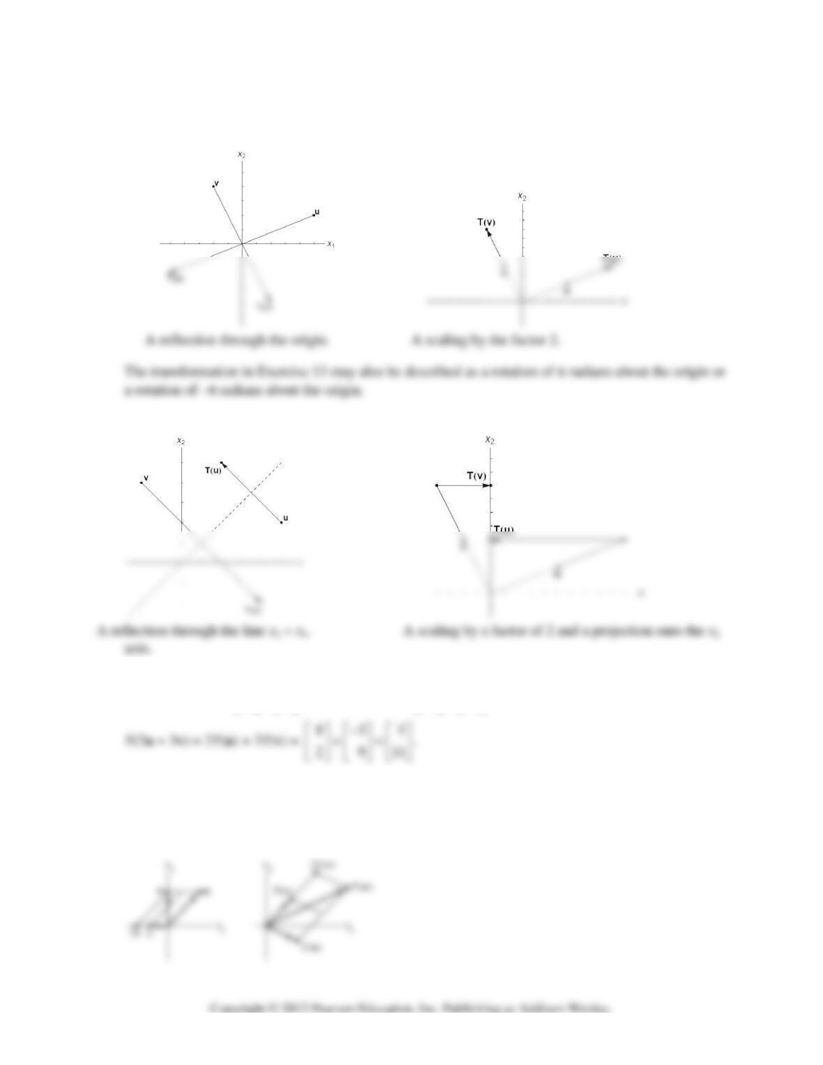
13. 14.
15. 16.
17. T(2u) = 2T(u) =
48
212
⎡⎤ ⎡⎤
=
⎢⎥ ⎢⎥
⎣⎦ ⎣⎦
, T(3v) = 3T(v) =
13
339
−−
⎡
⎤⎡⎤
=
⎢
⎥⎢⎥
⎣
⎦⎣⎦
, and
18. Draw a line through w parallel to v, and draw a line through w parallel to u. See the left part of the
figure below. From this, estimate that w = u + 2v. Since T is linear, T(w) = T(u) + 2T(v). Locate T(u)
and 2T(v) as in the right part of the figure and form the associated parallelogram to locate T(w).
19. All we know are the images of e
1
and e
2
and the fact that T is linear. The key idea is to write
x =
12
510
5353
301
.
=−=−
−
⎡⎤ ⎡⎤ ⎡⎤
⎢⎥ ⎢⎥ ⎢⎥
⎣⎦ ⎣⎦ ⎣⎦
ee
Then, from the linearity of T, write
20. Use the basic definition of Ax to construct A. Write
21. a. True. Functions from R
n
to R
m
are defined before Fig. 2. A linear transformation is a function
with certain properties.
22. a. True. See the subsection on Matrix Transformations.
b. True. See the subsection on Linear Transformations.
23. a. When b = 0, f (x) = mx. In this case, for all x,y in R and all scalars c and d,
f (cx + dy) = m(cx + dy) = mcx + mdy = c(mx) + d(my) = cf (x) + d f (y)
This shows that f is linear.
24. Let T(x) = Ax + b for x in R
n
. If b is not zero, T(0) = A0 + b = b
≠
0. Actually, T fails both