1.3 • Solutions 21
27.6 30.2 162 1.000 0 3.900
⎡⎤⎡⎤
29. The total mass is 4 + 2 + 3 + 5 = 14. So v = (4v
1
+2v
2
+ 3v
3
+ 5v
4
)/14. That is,
2 4 4 1 8 8 12 5 17 14 1.214
⎛⎞−−++
⎡⎤ ⎡⎤ ⎡⎤ ⎡⎤ ⎡ ⎤⎡ ⎤⎡ ⎤
30. Let m be the total mass of the system. By definition,
1
11 1
1()
k
kk k
m
m
mm
=++=++vv vv v“”
31. a. The center of mass is
08210/3
1111
114 2
3
⎛⎞
⎡⎤ ⎡⎤ ⎡⎤ ⎡ ⎤
⋅+⋅+⋅ =
⎜⎟
⎢⎥ ⎢⎥ ⎢⎥ ⎢ ⎥
⎣⎦ ⎣⎦ ⎣⎦ ⎣ ⎦
⎝⎠
.
b. The total mass of the new system is 9 grams. The three masses added, w
1
, w
2
, and w
3
, satisfy the
equation
() () ()
123
0822
1111
1142
9www
⎛⎞
⎡
⎤⎡⎤⎡⎤⎡⎤
+⋅ + +⋅ + +⋅ =
⎜⎟
⎢
⎥⎢⎥⎢⎥⎢⎥
⎣
⎦⎣⎦⎣⎦⎣⎦
⎝⎠
The condition w
1
+ w
2
+ w
3
= 6 and the vector equation above combine to produce a system of
three equations whose augmented matrix is shown below, along with a sequence of row
operations:
111 6 1116 1116
082 8~0828~0828
11412 0036 0012
⎡⎤⎡⎤⎡⎤
⎢⎥⎢⎥⎢⎥
⎢⎥⎢⎥⎢⎥
⎢⎥⎢⎥⎢⎥
⎣⎦⎣⎦⎣⎦
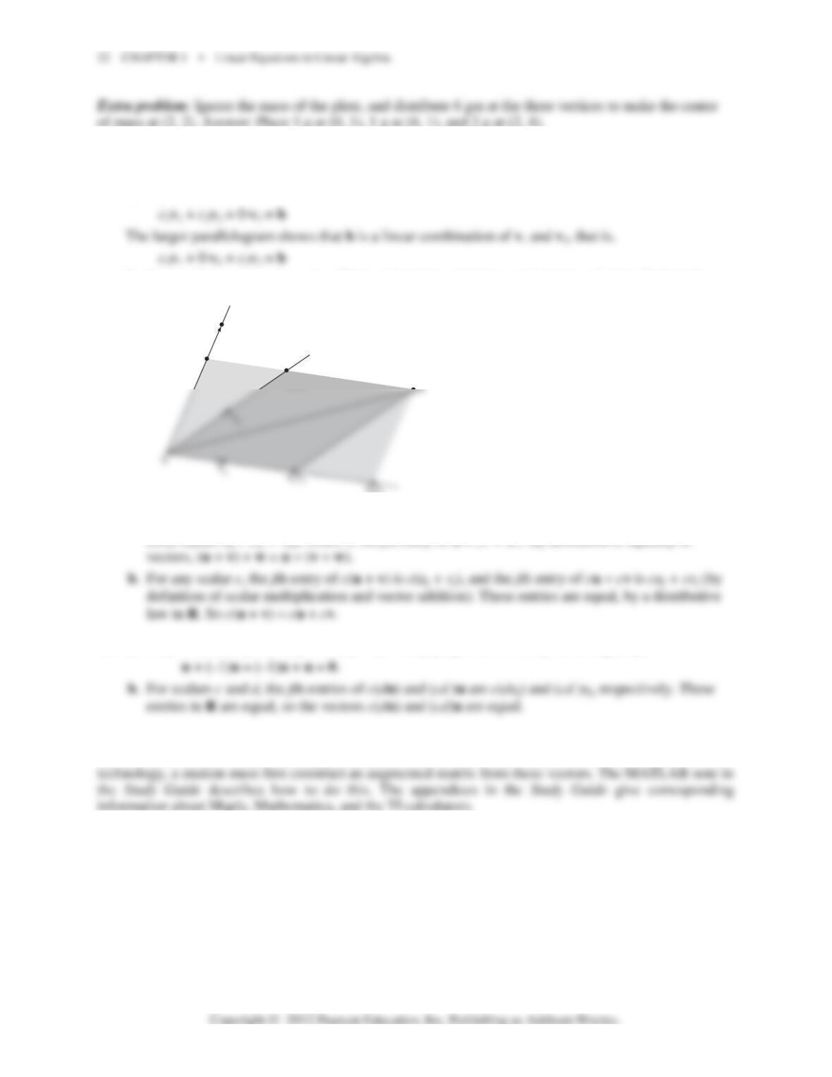
32. See the parallelograms drawn on the figure from the text that accompanies this exercise. Here c
1
, c
2
,
c
3
, and c
4
are suitable scalars. The darker parallelogram shows that b is a linear combination of v
1
and v
2
, that is
So the equation x
1
v
1
+ x
2
v
2
+ x
3
v
3
= b has at least two solutions, not just one solution. (In fact, the
equation has infinitely many solutions.)
33. a. For j = 1,…, n, the jth entry of (u + v) + w is (u
j
+ v
j
) + w
j
. By associativity of addition in R, this
entry equals u
+ (v
+ w
), which is the jth entry of u + (v + w). By definition of equality of
34. a. For j = 1,…, n, u
j
+ (–1)u
j
= (–1)u
j
+ u
j
= 0, by properties of R. By vector equality,
Note:
When an exercise in this section involves a vector equation, the corresponding technology data (in
the data files on the web) is usually presented as a set of (column) vectors. To use MATLAB or other
c
2
v
2
c
3
v
3
v
3
4
1
1.4 • Solutions 23
1.4 SOLUTIONS
Notes:
Key exercises are 1–20, 27, 28, 31 and 32. Exercises 29, 30, 33, and 34 are harder. Exercise 34
anticipates the Invertible Matrix Theorem but is not used in the proof of that theorem.
2. The matrix-vector Ax is not defined because the number of columns (1) in the 3×1 matrix A does not
match the number of entries (2) in the vector x.
12 1 2 2 6 4
−
⎡⎤ ⎡⎤⎡⎤⎡⎤⎡⎤⎡⎤
12 1(2)23 4
⋅− + ⋅
⎡⎤ ⎡ ⎤⎡⎤
1
13 4 1 3 4 164 3
⎡⎤
−−+−
1
⎡⎤
5. On the left side of the matrix equation, use the entries in the vector x as the weights in a linear
combination of the columns of the matrix A:
6. On the left side of the matrix equation, use the entries in the vector x as the weights in a linear
combination of the columns of the matrix A:
2321
−−
⎡⎤ ⎡⎤⎡ ⎤
7. The left side of the equation is a linear combination of three vectors. Write the matrix A whose
columns are those three vectors, and create a variable vector x with three entries:
24 CHAPTER 1 • Linear Equations in Linear Algebra
⎢
⎢
⎣
457 457
138 138
⎡⎤−−
⎡⎤⎡⎤⎡⎤ ⎡ ⎤
⎢⎥
⎢⎥⎢⎥⎢⎥ ⎢ ⎥
−−−−
⎢⎥
⎢⎥⎢⎥⎢⎥ ⎢ ⎥
1
x
⎡
⎤
⎢
⎥
1
457 6
138 8
x
−
⎡⎤⎡⎤
⎡⎤
⎢⎥⎢⎥
−− −
Note:
The skill of writing a vector equation as a matrix equation will be important for both theory and
application throughout the text. See also Exercises 27 and 28.
8. The left side of the equation is a linear combination of four vectors. Write the matrix A whose
columns are those four vectors, and create a variable vector with four entries:
2140 2140
4532 4532
A⎡⎤−− −−
⎡⎤⎡⎤⎡⎤⎡⎤ ⎡ ⎤
==
⎢⎥
⎢⎥⎢⎥⎢⎥⎢⎥ ⎢ ⎥
−−
⎣⎦⎣⎦⎣⎦⎣⎦ ⎣ ⎦
⎣⎦
, and
1
2
3
⎢
⎣
z
z
z
⎡
⎤
⎢
⎥
⎢
⎥
=
⎢
⎥
⎢
⎥
z
. Then the equation Az = b
4
2
3
4
3
4
9. The system has the same solution set as the vector equation
123
51 38
02 40
xx x
−
⎡⎤ ⎡⎤ ⎡ ⎤ ⎡⎤
++ =
⎢⎥ ⎢⎥ ⎢ ⎥ ⎢⎥
⎣⎦ ⎣⎦ ⎣ ⎦ ⎣⎦
and this equation has the same solution set as the matrix equation
10. The system has the same solution set as the vector equation
418
−
⎡⎤ ⎡ ⎤ ⎡⎤
1.4 • Solutions 25
41 8
−
⎡⎤ ⎡⎤
11. To solve Ax = b, row reduce the augmented matrix [a
1
a
2
a
3
b] for the corresponding linear
system:
1342 1342 1342 1302 10011
−− −− −− − −
⎡⎤⎡⎤⎡⎤⎡⎤⎡⎤
12. To solve Ax = b, row reduce the augmented matrix [a
1
a
2
a
3
b] for the corresponding linear
system:
1211 1211 1211 1211
3422~0215~0888~0111
−−−−
⎡⎤⎡⎤⎡⎤⎡⎤
⎢⎥⎢⎥⎢⎥⎢⎥
−− − − − −
13. The vector u is in the plane spanned by the columns of A if and only if u is a linear combination of
the columns of A. This happens if and only if the equation Ax = u has a solution. (See the box
preceding Example 3 in Section 1.4.) To study this equation, reduce the augmented matrix [A u]
350 114 11 4 114
−
14. Reduce the augmented matrix [A u] to echelon form:
25 1 4 12 0 4 12 0 4 12 0 4
−
⎡⎤⎡⎤⎡⎤⎡⎤
26 CHAPTER 1 • Linear Equations in Linear Algebra
15. The augmented matrix for Ax = b is
1
2
31
93
b
b
−
⎡⎤
⎢⎥
−
⎣⎦
, which is row equivalent to
1
21
31
00 3
b
bb
−
⎡⎤
⎢⎥
+
⎣⎦
.
16. Row reduce the augmented matrix [A b]:
1
2
3
121
220, .
413
b
Ab
b
−−
⎡
⎤⎡⎤
⎢
⎥
⎢⎥
=− =
⎢
⎥
⎢⎥
⎢
⎥⎢⎥
−
⎣⎦
⎣
⎦
b
11
121 12 1
bb
−− −−
⎡⎤⎡ ⎤
17. Row reduction shows that only three rows of A contain a pivot position:
1303 1303 1303 1303
⎡⎤⎡⎤⎡⎤⎡⎤
⎢⎥⎢⎥⎢⎥⎢⎥
18. Row reduction shows that only three rows of B contain a pivot position:
14 1 2 14 1 2 14 1 2 1 4 1 2
⎡⎤⎡ ⎤⎡⎤⎡ ⎤
⎢⎥⎢ ⎥⎢⎥⎢ ⎥
19. The work in Exercise 17 shows that statement (d) in Theorem 4 is false. So all four statements in
1.4 • Solutions 27
20. The work in Exercise 18 shows that statement (d) in Theorem 4 is false. So all four statements in
21. Row reduce the matrix [v
1
v
2
v
3
] to determine whether it has a pivot in each row.
10 1 10 1 10 1 101
010 010 010 010
⎡ ⎤⎡⎤⎡⎤⎡⎤
⎢ ⎥⎢⎥⎢⎥⎢⎥
−−−
22. Row reduce the matrix [v
1
v
2
v
3
] to determine whether it has a pivot in each row.
004 396
−−
⎡⎤⎡⎤
23. a. False. See the paragraph following equation (3). The text calls Ax = b a matrix equation.
b. True. See the box before Example 3.
24. a. True. This statement is in Theorem 3. However, the statement is true without any “proof”
because, by definition, Ax is simply a notation for x
1
a
1
+ ⋅ ⋅ ⋅ + x
n
a
n
, where a
1
, …, a
n
are the
25. By definition, the matrix-vector product on the left is a linear combination of the columns of the
26. The equation in x
1
and x
2
involves the vectors u, v, and w, and it may be viewed as
27. The matrix equation can be written as c
1
v
1
+ c
2
v
2
+ c
3
v
3
+ c
4
v
4
+ c
5
v
5
= v
6
, where
28. Place the vectors q
1
, q
2
, and q
3
into the columns of a matrix, say, Q and place the weights x
1
, x
2
, and
x
3
into a vector, say, x. Then the vector equation becomes
29. Start with any 3×3 matrix B in echelon form that has three pivot positions. Perform a row operation
(a row interchange or a row replacement) that creates a matrix A that is not in echelon form. Then A
30. Start with any nonzero 3×3 matrix B in echelon form that has fewer than three pivot positions.
31. A 3×2 matrix has three rows and two columns. With only two columns, A can have at most two pivot
columns, and so A has at most two pivot positions, which is not enough to fill all three rows. By
32. A set of three vectors in R
4
cannot span R
4
. Reason: the matrix A whose columns are these three
vectors has four rows. To have a pivot in each row, A would have to have at least four columns (one
33. If the equation Ax = b has a unique solution, then the associated system of equations does not have
any free variables. If every variable is a basic variable, then each column of A is a pivot column. So
⎢
⎢
⎢
⎢
⎢
⎣
100
⎡
⎤
34. Given Au
1
= v
1
and Au
2
= v
2
, you are asked to show that the equation Ax = w has a solution, where
35. Suppose that y and z satisfy Ay = z. Then 5z = 5Ay. By Theorem 5(b), 5Ay = A(5y). So 5z = A(5y),
36. If the equation Ax = b has a unique solution, then the associated system of equations does not have
any free variables. If every variable is a basic variable, then each column of A is a pivot column. So
⎢
⎢
⎢
⎢
⎣
1000
⎡
⎤
each row. By Theorem 4, the columns of A span R
4
.
72587258725 8
−− −
⎡⎤⎡ ⎤⎡ ⎤
⎣⎦⎣ ⎦⎣ ⎦
7258
−
⎡⎤
⎢⎥
not have a pivot in every row, so its columns do not span R
4
, by Theorem 4.
4518 4 5 1 8 4 5 1 8
−− −− −−
⎡⎤⎡ ⎤⎡ ⎤
With pivots only in the first three rows, the original matrix has columns that do not span R
4
, by
Theorem 4.
10 7 1 4 6 10 7 1 4 6
846103 0 8/5 26/534/5 9/5
−−
⎡⎤⎡ ⎤
⎢⎥⎢ ⎥
−−−− −−−
The original matrix has a pivot in every row, so its columns span R
4
, by Theorem 4.
5 11 6 7 12 5 11 6 7 12
−− − −
⎡⎤⎡ ⎤
30 CHAPTER 1 • Linear Equations in Linear Algebra
5 11 6 7 12 5 11 6 7 12
0 62/5 62/5 19/5 39/5 0 62/5 62/5 19/5 39/5
−− −−
⎡⎤⎡⎤
⎢⎥⎢⎥
−− −−
41. [M] Examine the calculations in Exercise 39. Notice that the fourth column of the original matrix,
say A, is not a pivot column. Let A
o
be the matrix formed by deleting column 4 of A, let B be the
echelon form obtained from A, and let B
o
be the matrix obtained by deleting column 4 of B. The
Note:
Exercises 41 and 42 help to prepare for later work on the column space of a matrix. (See Section
2.9 or 4.6.) The Study Guide points out that these exercises depend on the following idea, not explicitly
42. [M] Examine the calculations in Exercise 40. The third column of the original matrix, say A, is not a
pivot column. Let A
o
be the matrix formed by deleting column 3 of A, let B be the echelon form
obtained from A, and let B
o
be the matrix obtained by deleting column 3 of B. The sequence of row
operations that reduces A to B also reduces A
o
to B
o
. Since B
o
is in echelon form, it shows that A
o
has
a pivot position in each row. Therefore, the columns of A
o
span R
4
.
Notes:
At the end of Section 1.4, the Study Guide gives students a method for learning and mastering
linear algebra concepts. Specific directions are given for constructing a review sheet that connects the
basic definition of “span” with related ideas: equivalent descriptions, theorems, geometric interpretations,
special cases, algorithms, and typical computations. I require my students to prepare such a sheet that
reflects their choices of material connected with “span”, and I make comments on their sheets to help
1.5 • Solutions 31
If an interchange is required, I can insert a command such as B = swap(B,2,5) . The command
bgauss uses the left-most nonzero entry in a row to produce zeros above that entry. This command,
1.5 SOLUTIONS
Notes
: The geometry helps students understand Span{u, v}, in preparation for later discussions of sub-
spaces. The parametric vector form of a solution set will be used throughout the text. Figure 6 will appear
again in Sections 2.9 and 4.8.
For solving homogeneous systems, the text recommends working with the augmented matrix, al-
though no calculations take place in the augmented column. See the Study Guide comments on Exercise 7
that illustrate two common student errors.
1. Reduce the augmented matrix to echelon form and circle the pivot positions. If a column of the
coefficient matrix is not a pivot column, the corresponding variable is free and the system of
equations has a nontrivial solution. Otherwise, the system has only the trivial solution.
258025802580
−−−
⎡⎤⎡⎤⎡⎤
The variable x
3
is free, so the system has a nontrivial solution.
1230 1230
−−
⎡⎤⎡⎤
There is no free variable; the system has only the trivial solution.
34 80 3 4 80
−− − −
⎡⎤⎡ ⎤
1.2.
32 CHAPTER 1 • Linear Equations in Linear Algebra
5320 5 3 20
−−
⎡⎤⎡ ⎤
solutions. As in Exercise 3, row operations are unnecessary.
2 2 40 2 2 40 1120 1010
⎡⎤⎡⎤⎡⎤⎡⎤
13
0
xx
+=
⎢
⎢
⎢
⎣
13
1
xx
−−
⎡⎤⎡ ⎤
⎡
⎤
12 30 1 2 30 12 30 10 10
−−−−
⎡⎤⎡⎤⎡⎤⎡⎤
⎡
⎢
⎢
⎢
⎣
13
0
xx
−=
7.
13370 10980
~
01 450 01 4 50
−−
⎡⎤⎡ ⎤
⎢⎥⎢ ⎥
−−
⎣⎦⎣ ⎦
.
134
234
980
450
xxx
xxx
+−=
−+=
The basic variables are x
1
and x
2
, with x
3
and x
4
free. Next, x
1
= –9x
3
+ 8x
4
, and x
2
= 4x
3
– 5x
4
. The
general solution is
134 4
3
98 8
998
xxx x
x
−+ −−
⎡⎤⎡ ⎤ ⎡ ⎤
⎡⎤ ⎡⎤⎡⎤
8.
13850 10270
~
−− −−
⎡⎤⎡⎤
.
134
270
xxx
−−=
1.5 • Solutions 33
134 4
3
27 7
227
xxx x
x
+
⎡⎤⎡ ⎤ ⎡ ⎤
⎡⎤ ⎡⎤⎡⎤
9.
~~~
2420 2420 0020 0010
⎢⎥⎢⎥⎢⎥⎢⎥
−− −−
⎣⎦⎣⎦⎣⎦⎣⎦
12
20
xx
−=
10.
1 40 40 1 4040 14040 10040
~~~
2 8 0 80 2 8 080 0 1 000 0 1 000
−− −
⎡⎤⎡⎤⎡⎤⎡⎤
⎢⎥⎢⎥⎢⎥⎢⎥
−−
⎣⎦⎣⎦⎣⎦⎣⎦
The basic variables are x
1
and x
2
, so x
3
and x
4
are free. (Note that x
3
is not zero.) Also, x
1
= –4x
4
. The
general solution is
⎢
⎢
⎢
⎢
⎣
14 4
44
004
xx x
−− −
⎡⎤⎡ ⎤ ⎡ ⎤
⎡
⎤⎡⎤⎡⎤
11.
1420350 1420070 1400050
0010010 0010010 0010010
−− − −− −
⎡⎤⎡⎤⎡⎤
⎢⎥⎢⎥⎢⎥
−−−
The basic variables are x
1
, x
3
, and x
5
. The remaining variables are free. In particular, x
4
is free (and
not zero as some may assume). The solution is x
1
= 4x
2
– 5x
6
, x
3
= x
6
, x
5
= 4x
6
, with x
2
, x
4
, and x
6
free.
In parametric vector form,
34 CHAPTER 1 • Linear Equations in Linear Algebra
⎢
⎢
⎢
⎢
⎢
⎢
⎢
⎣
126 6
2
22 2
45 5
40 40
0
010
xxx x
x
xx x
−−
⎡⎤⎡ ⎤ ⎡ ⎤
⎡⎤⎡⎤ ⎡⎤
⎢⎥⎢ ⎥ ⎢ ⎥
⎢⎥⎢⎥ ⎢⎥
5
0
−
⎡
⎤⎡⎤
⎢
⎥⎢⎥
Note
: The Study Guide discusses two mistakes that students often make on this type of problem.
12.
1 2 3 6 5 00 1 2 3 6 500 1 2 30 2900
0 0 0 1 4 60 0 0 0 1 400 0 0 0 1 400
−− −− −
⎡⎤⎡⎤⎡⎤
⎢⎥⎢⎥⎢⎥
−
123 5
23 29 0
xxx x
−+ + =
The basic variables are x
1
, x
4
, and x
6
; the free variables are x
2
, x
3
, and x
5
. The general solution is
x
1
= 2x
2
– 3x
3
– 29x
5
, x
4
= – 4x
5
, and x
6
= 0. In parametric vector form, the solution is
123 5 2 3 5
⎢
333
2
455
⎥
⎥
⎥
⎣
2 3 29 2 3 29 2
000
40040
xxx x x x x
xxx
x
xxx
−− − −
⎡⎤⎡⎤⎡⎤⎡⎤⎡⎤⎡⎤
⎢⎥⎢⎥⎢⎥⎢⎥⎢⎥⎢⎥
⎢⎥⎢⎥⎢⎥⎢⎥⎢⎥⎢⎥
== = + + =
⎢⎥⎢⎥⎢⎥⎢⎥⎢⎥⎢⎥
−−
⎢⎥⎢⎥⎢⎥⎢⎥⎢⎥⎢⎥
x
35
329
10
04
xx
−−
⎡
⎤⎡⎤
⎢
⎥⎢⎥
⎢
⎥⎢⎥
++
⎢
⎥⎢⎥
−
⎢
⎥⎢⎥
13. To write the general solution in parametric vector form, pull out the constant terms that do not
involve the free variable:
⎡
⎢
⎢
⎢
⎣
⎡
⎢
⎢
⎢
⎣
13 3
54 5 4 5 4
xx x
+
⎡⎤⎡ ⎤ ⎡ ⎤
⎡⎤ ⎡⎤ ⎡⎤
14. To write the general solution in parametric vector form, pull out the constant terms that do not
involve the free variable:
14 4
55
005
32 2
332
xx x
xx xxx
⎡⎤⎡ ⎤ ⎡ ⎤
⎡⎤ ⎡⎤ ⎡ ⎤
⎢⎥⎢ ⎥ ⎢ ⎥
⎢⎥ ⎢⎥ ⎢ ⎥
−− −
The solution set is the line through p in the direction of q.
15. Solve x
1
+ 5x
2
– 3x
3
= –2 for the basic variable: x
1
= –2 – 5x
2
+ 3x
3
, with x
2
and x
3
free. In vector
form, the solution is
123 23
25 3 2 5 3 2 5 3
xxx xx
−− + − − − −
⎡⎤⎡ ⎤ ⎡ ⎤⎡⎤⎡ ⎤ ⎡⎤ ⎡⎤ ⎡⎤
The solution of x
1
+ 5x
2
– 3x
3
= 0 is x
1
= – 5x
2
+ 3x
3
, with x
2
and x
3
free. In vector form,
12323
53 5 3 5 3
xxxxx
−+ − −
⎡⎤⎡ ⎤ ⎡ ⎤⎡⎤ ⎡⎤⎡⎤
The solution set of the homogeneous equation is the plane through the origin in R
3
spanned by
u and v. The solution set of the nonhomogeneous equation is parallel to this plane and passes through
2
−
⎡⎤
16. Solve x
1
– 2x
2
+ 3x
3
= 4 for the basic variable: x
1
= 4 + 2x
2
– 3x
3
, with x
2
and x
3
free. In vector form,
the solution is
123 23
42 3 4 2 3 4 2 3
xxx xx
+− − −
⎡⎤⎡ ⎤ ⎡ ⎤⎡⎤ ⎡ ⎤ ⎡⎤ ⎡⎤ ⎡ ⎤
The solution of x
1
– 2x
2
+ 3x
3
= 0 is x
1
= 2x
2
– 3x
3
, with x
2
and x
3
free. In vector form,
1232 3
23 2 3 2 3
xxxx x
−− −
⎡⎤⎡ ⎤ ⎡ ⎤⎡⎤ ⎡⎤ ⎡⎤
17. Row reduce the augmented matrix for the system:
224 8 2248 2248 1124 1018
44816~0000~03312~0114~0114
⎡ ⎤⎡⎤⎡⎤⎡⎤⎡⎤
⎢ ⎥⎢⎥⎢⎥⎢⎥⎢⎥
−−−− −− − −
00
=
13 3
23 3 3
⎢
⎢
⎣
88 81
44 41
xx x
xx x x
−− −
⎡⎤⎡ ⎤ ⎡ ⎤
⎡
⎤⎡⎤⎡⎤
⎢⎥⎢ ⎥ ⎢ ⎥
⎢
⎥⎢⎥⎢⎥
= =−− =− +− =− + −
x
18. Row reduce the augmented matrix for the system:
1235 1235 1235 1017
21 313~0 3 3 3~0 1 1 1~0 1 1 1
−−−−
⎡⎤⎡⎤⎡⎤⎡⎤
⎢⎥⎢⎥⎢⎥⎢⎥
− − −− −−
13 3
23 3 3
⎢
⎣
77 71
11 11
xx x
xx x x
+
⎡⎤⎡ ⎤ ⎡⎤
⎡
⎤⎡⎤⎡⎤
⎢⎥⎢ ⎥ ⎢⎥
⎢
⎥⎢⎥⎢⎥
==−+=−+=−+
⎢⎥⎢ ⎥ ⎢⎥
⎢
⎥⎢⎥⎢⎥
x
19. The line through a parallel to b can be written as x = a + t b, where t represents a parameter:
x =
1
25
xt
−−
⎡⎤⎡ ⎤ ⎡⎤
=+
⎢⎥⎢⎥ ⎢⎥
, or
1
25
xt
=− −
⎧
⎨=
1.5 • Solutions 37
21. The line through p and q is parallel to q – p. So, given
34
and
⎣
⎡
⎢
⎣
⎡
⎤⎡⎤
==
⎢
⎥⎢⎥
pq
, form
22. The line through p and q is parallel to q – p. So, given
30
and
23
−
⎡
⎤⎡⎤
==
⎢
⎥⎢⎥
−
⎣
⎦⎣⎦
pq
, form
⎡
⎢
⎣
23. a. True. See the first paragraph of the subsection titled Homogeneous Linear Systems.
b. False. The equation Ax = 0 gives an implicit description of its solution set. See the subsection
entitled Parametric Vector Form.
24. a. False. The trivial solution is always a solution to a homogeneous system of linear equations.
b. False. A nontrivial solution of Ax = 0 is any nonzero x that satisfies the equation. See the
25. Suppose p satisfies Ax = b. Then Ap = b. Theorem 6 says that the solution set of Ax = b equals the
set S ={w : w = p + v
h
for some v
h
such that Av
h
= 0}. There are two things to prove: (a) every vector
in S satisfies Ax = b, (b) every vector that satisfies Ax = b is in S.
a. Let w have the form w = p + v
h
, where Av
h
= 0. Then
So every vector of the form p + v
h
satisfies Ax = b.
b. Now let w be any solution of Ax = b, and set v
= w − p. Then
26. When A is the 3×3 zero matrix, every x in R
3
satisfies Ax = 0. So the solution set is all vectors in R
3
.
27. (Geometric argument using Theorem 6.) Since Ax = b is consistent, its solution set is obtained by
translating the solution set of Ax = 0, by Theorem 6. So the solution set of Ax = b is a single vector if
38 CHAPTER 1 • Linear Equations in Linear Algebra
28. a. When A is a 3×3 matrix with three pivot positions, the equation Ax = 0 has no free variables and
hence has no nontrivial solution.
29. a. When A is a 4×4 matrix with three pivot positions, the equation Ax = 0 has three basic variables
andone free variable. So Ax = 0 has a nontrivial solution.
30. a. When A is a 2×5 matrix with two pivot positions, the equation Ax = 0 has two basic variables and
three free variables. So Ax = 0 has a nontrivial solution.
31. a. When A is a 3×2 matrix with two pivot positions, each column is a pivot column. So the equation
Ax = 0 has no free variables and hence no nontrivial solution.
32. No. If the solution set of Ax = b contained the origin, then 0 would satisfy A0= b, which is not true
since b is not the zero vector.
34. Look for A = [a
1
a
2
a
3
] such that 2 a
1
– 1 a
2
+ 1 a
3
= 0. That is, construct A so that subtracting the
third column from the second column is twice the first column.
35. Look at
12
13
721
26
xx
−−
⎡⎤ ⎡⎤
⎢⎥ ⎢⎥
+
⎢⎥ ⎢⎥
⎢⎥ ⎢⎥
−−
⎣⎦ ⎣⎦
and notice that the second column is 3 times the first. So suitable values
36. Inspect how the columns a
1
and a
2
of A are related. The second column is –2/3 times the first. Put
37. Since the solution set of Ax = 0 contains the point (4,1), the vector x = (4,1) satisfies Ax = 0. Write
this equation as a vector equation, using a
1
and a
2
for the columns of A:
4
a
1
+ 1 a
2
= 0
Then a
2
= –4a
1
. So choose any nonzero vector for the first column of A and multiply that column by
Note
: In the Study Guide, a “Checkpoint” for Section 1.5 will help students with Exercise 37.
38. If w satisfies Ax = 0, then Aw = 0. For any scalar c, Theorem 5(b) in Section 1.4 shows that
39. Suppose Av = 0 and Aw = 0. Then, since A(v + w) = Av + Aw by Theorem 5(a) in Section 1.4,
A(v + w) = Av + Aw = 0 + 0 = 0.
40. No. If Ax = b has no solution, then A cannot have a pivot in each row. Since A is 3×3, it has at most
two pivot positions. So the equation Ax = y for any y has at most two basic variables and at least one
1.6 SOLUTIONS
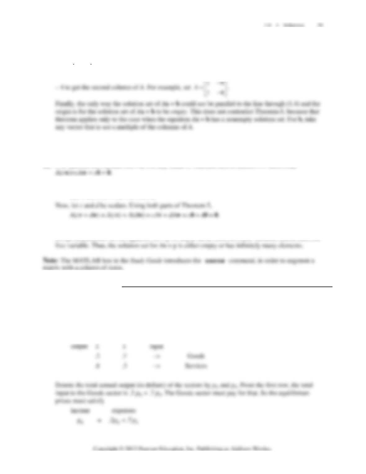
1. Fill in the exchange table one column at a time. The entries in a column describe where a sector’s
output goes. The decimal fractions in each column sum to 1.
Distribution of
Output From:
Goods Services Purchased by:
40 CHAPTER 1 • Linear Equations in Linear Algebra
From the second row, the input (that is, the expense) of the Services sector is .8 p
G
+ .3 p
S
.
The equilibrium equation for the Services sector is
income expenses
=.8 .3
SGS
ppp+
Row reduce the augmented matrix:
.8 .7 0 .8 .7 0 1 .875 0
~~
.8 .7 0 0 0 0 0 0 0
−−−
⎡⎤⎡⎤⎡⎤
⎢⎥⎢⎥⎢⎥
−
⎣⎦⎣⎦⎣⎦
The general solution is p
G
= .875 p
S
, with p
S
free. One equilibrium solution is p
S
= 1000 and p
G
=
875. If one uses fractions instead of decimals in the calculations, the general solution would be
2. Take some other value for p
S
, say 200 million dollars. The other equilibrium prices are then
p
C
= 188 million, p
E
= 170 million. Any constant nonnegative multiple of these prices is a set of
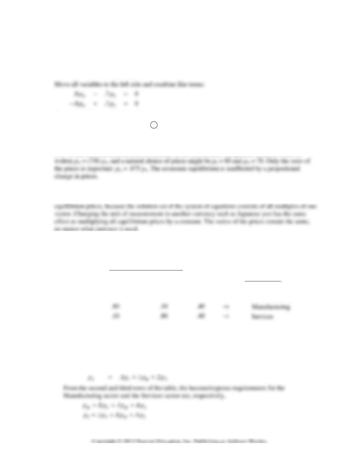
3. a. Fill in the exchange table one column at a time. The entries in a column describe where a sector’s
output goes. The decimal fractions in each column sum to 1.
Distribution of Output From :
Purchased by :
Fuels and Power Manufacturing Services
output input
.10 .10 .20 Fuels and Power
↓↓↓
→
b. Denote the total annual output (in dollars) of the sectors by p
F
, p
M
, and p
S
. From the first row of
the table, the total input to the Fuels & Power sector is .1p
F
+ .1p
M
+ .2p
S
. So the equilibrium
prices must satisfy