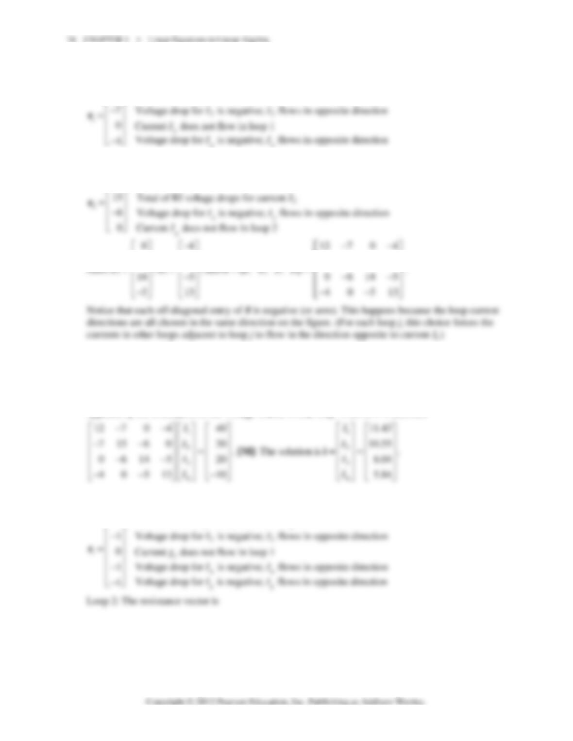
7. Loop 1: The resistance vector is
1
Total of RI voltage drops for current
12
I
⎡⎤
Loop 2: The resistance vector is
1
1
Voltage drop for is negative; flows in opposite direction
7
II
⎡⎤
−
⎢
⎢
⎢
⎣
⎢
⎢
⎢
⎣
6
⎢⎥
−
⎢⎥
0
⎡
⎤
⎢
⎥
⎢
⎥
715 6 0
⎡
⎤
⎢
⎥
−−
⎢
⎥
Next, set v
40
30
20
10
⎡⎤
⎢⎥
⎢⎥
=⎢⎥
⎢⎥
−
⎢⎥
⎣⎦
. Note the negative voltage in loop 4. The current direction chosen in loop 4 is
opposed by the orientation of the voltage source in that loop. Thus Ri = v becomes
⎡
⎢
⎢
⎢
⎢
⎢
⎣
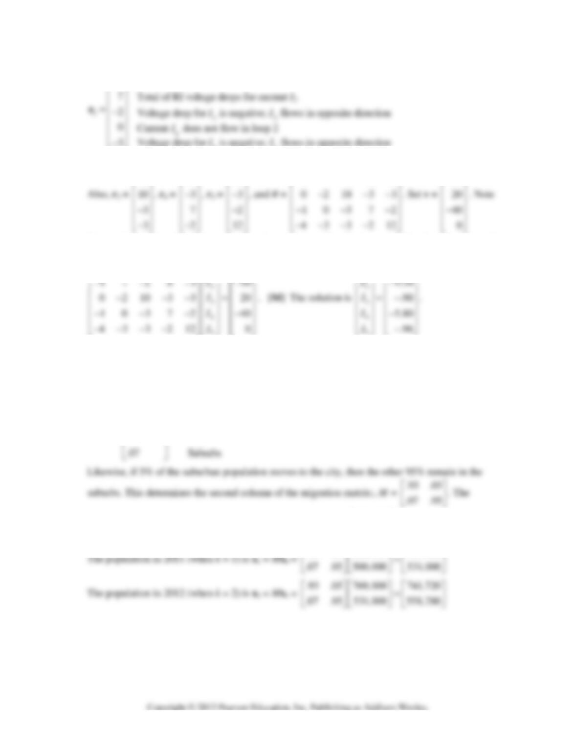
8. Loop 1: The resistance vector is
1
Total of RI voltage drops for current
9
I
⎡⎤
1.10 • Solutions 75
11
Voltage drop for is negative; flows in opposite direction
1
II
⎡⎤
−
55
⎢
⎢
⎢
⎢
⎢
⎣
⎢
⎢
⎢
⎢
⎢
⎣
0
2
⎡⎤
⎢⎥
−
1
0
−
⎡
⎤
⎢
⎥
4
3
−
⎡⎤
⎢⎥
−
91014
17 20 3
−−−
⎡
⎤
⎢
⎥
−−−
50
30
⎡⎤
⎢⎥
−
the negative voltages for loops where the chosen current direction is opposed by the orientation of
the voltage source in that loop. Thus Ri = v becomes:
⎢
⎢
⎢
⎢
⎢
⎣
1
91014 50
I
−−−
⎡⎤
⎡⎤⎡⎤
⎢⎥
⎢⎥⎢⎥
1
4.00
I
⎡⎤
⎡
⎤
⎢⎥
⎢
⎥
9. The population movement problems in this section assume that the total population is constant, with
no migration or immigration. The statement that “about 7% of the city’s population moves to the
suburbs” means also that the rest of the city’s population (93%) remain in the city. This determines
the entries in the first column of the migration matrix (which concerns movement from the city).
From:
City Suburbs To:
.93 City
⎡
⎢
⎣
⎡⎤
difference equation is x
k+1
= Mx
k
for k = 0, 1, 2, …. Also, x
0
= 800,000
500,000
⎡
⎤
⎢
⎥
⎣
⎦
⎢
⎣
⎡
⎢
⎣
⎡
⎤⎡ ⎤ ⎡ ⎤
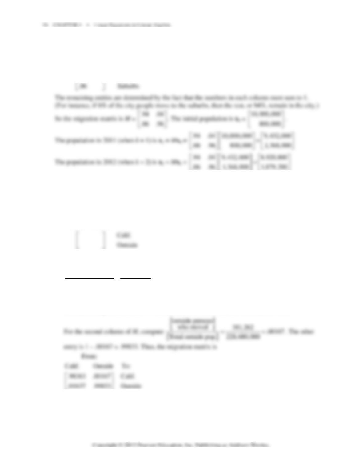
10. The data in the first sentence implies that the migration matrix has the form:
From:
City Suburbs To:
.04 City
⎡⎤
11. The problem concerns two groups of people–those living in California and those living outside
California (and in the United States). It is reasonable, but not essential, to consider the people living
inside California first. That is, the first entry in a column or row of a vector will concern the people
living in California. With this choice, the migration matrix has the form:
From:
Calif. Outside To:
a. For the first column of the migration matrix M, compute
{
}
{}
Calif. persons
who moved 516,100 .016372
Total Calif. pop. 31,524,000
==
The other entry in the first column is 1 – .016372 = .983628. The exercise requests that 5 decimal
places be used. So this number should be rounded to .98363. Whatever number of decimal places
is used, it is important that the two entries sum to 1. So, for the first fraction, use .01637.
⎣⎦
b. [M] The initial vector is x
0
= (31.524, 228.680), with data in millions of persons. Since x
0
describes the population in 1994, and x
1
describes the population in 1995, the vector x
6
describes
the projected population for the year 2000, assuming that the migration rates remain constant and
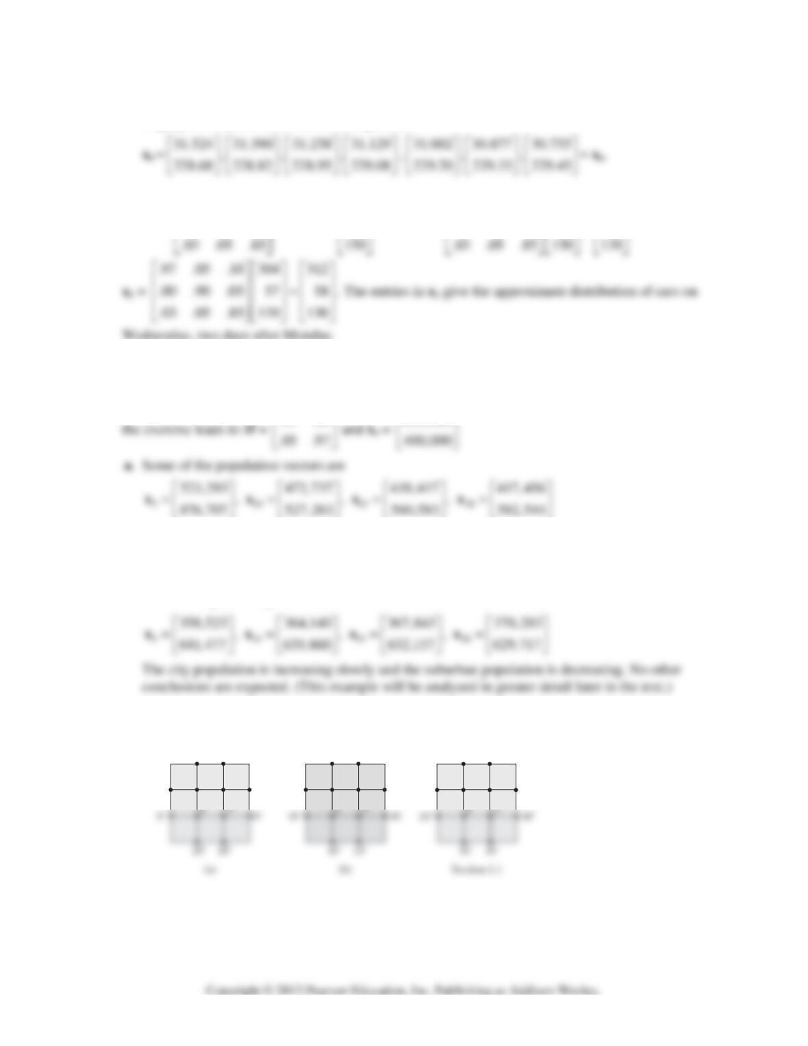
1.10 • Solutions 77
there are no deaths, births, or migration. Here are the vectors x
0
through x
6
with the first 5 figures
displayed. Numbers are in millions of persons:
12. Set M =
0
.97 .05 .10 295
.00 .90 .05 and 55
⎢
⎣
⎡⎤⎡⎤
⎢⎥⎢⎥
=
⎢⎥⎢⎥
x
. Then x
1
=
.97 .05 .10 295 304
.00 .90 .05 55 57
⎡
⎤⎡ ⎤ ⎡ ⎤
⎢
⎥⎢ ⎥ ⎢ ⎥
≈
⎢
⎥⎢ ⎥ ⎢ ⎥
, and
13. [M] The order of entries in a column of a migration matrix must match the order of the columns. For
instance, if the first column concerns the population in the city, then the first entry in each column
must be the fraction of the population that moves to (or remains in) the city. In this case, the data in
⎢
⎣
⎡⎤
⎡
⎤
The data here shows that the city population is declining and the suburban population is
increasing, but the changes in population each year seem to grow smaller.
b. When x
0
= 350,000
650,000
⎡⎤
⎢⎥
⎣⎦
, the situation is different. Now
14. Here are Figs. (a) and (b) for Exercise 13, followed by the figure for Exercise 34 in Section 1.1:
10˚
40˚
20˚ 20˚
12
0˚
0˚
20˚ 20˚
12
10˚
40˚
0˚ 0˚
12
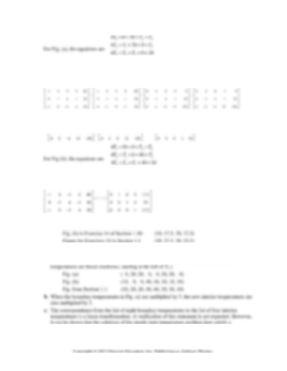
413
40 20
TTT
=+ + +
To solve the system, rearrange the equations and row reduce the augmented matrix. Interchanging
rows 1 and 4 speeds up the calculations. The first five steps are shown in detail.
4 1 0 1 20 1 0 1 4 20 1 0 1 4 20 1 0 1 4 20
− − −− −− −−
⎡⎤⎡ ⎤⎡⎤⎡⎤
10 1 4 20 10 1 4 20 100010
01 0 1 0 010 1 0 010010
~~~
004220 004220 001010
~
−− −−
−−
⋅⋅⋅
−−
⎡⎤⎡⎤⎡⎤
⎢⎥⎢⎥⎢⎥
⎢⎥⎢⎥⎢⎥
⎢⎥⎢⎥⎢⎥
413
410 10
TTT
=+++
Rearrange the equations and row reduce the augmented matrix:
4 1 0 1 10 1 0 0 0 10
−−
⎡⎤⎡⎤
a. Here are the solution temperatures for the three problems studied:
Fig. (a) in Exercise 14 of Section 1.10: (10, 10, 10, 10)
When the solutions are arranged this way, it is evident that the third solution is the sum of the first
two solutions. What might not be so evident is that list of boundary temperatures of the third
problem is the sum of the lists of boundary temperatures of the first two problems. (The
superposition principle. The system of equations that approximate the interior temperatures can
Chapter 1 • Supplementary Exercises 79
be written in the form Ax = b, where A is determined by the arrangement of the four interior
points on the plate and b is a vector in R
4
determined by the boundary temperatures.
Chapter 1 SUPPLEMENTARY EXERCISES
1. a. False. (The word “reduced” is missing.) Counterexample:
⎡⎤ ⎡ ⎤ ⎡⎤
b. False. Counterexample: Let A be any n×n matrix with fewer than n pivot columns. Then the
c. True. If a linear system has more than one solution, it is a consistent system and has a free
variable. By the Existence and Uniqueness Theorem in Section 1.2, the system has infinitely
many solutions.
d. False. Counterexample: The following system has no free variables and no solution:
12
2
1
5
xx
x
+=
=
but not every matrix equation Ax = b is consistent.
i. True. If A is row equivalent to B, then A can be transformed by elementary row operations first
into B and then further transformed into the reduced echelon form U of B. Since the reduced
echelon form of A is unique, it must be U.
j. False. Every equation Ax = 0 has the trivial solution whether or not some variables are free.
previous question. Since the row operations that transform B into I
3
are reversible, A can be
transformed first into I
3
and then into B.
o. True. The reason is essentially the same as that given for question f.
1
2
3
4
1
2
3
4
a pivot position in each of its five rows, which is impossible since A has only four columns.
t. True. The vector –u is a linear combination of u and v, namely, –u = (–1)u + 0v.
u. False. If u and v are multiples, then Span{u, v} is a line, and w need not be on that line.
v. False. Let u and v be any linearly independent pair of vectors and let w = 2v. Then w = 0u + 2v,
“transformation” in Section 1.8), and a linear transformation is a special type of transformation.
y. True. For the transformation x 6 Ax to map R
5
onto R
6
, the matrix A would have to have a pivot
in every row and hence have six pivot columns. This is impossible because A has only five
columns.
2. If a ≠ 0, then x = b/a; the solution is unique. If a = 0, and b ≠ 0, the solution set is empty, because
0x = 0 ≠ b. If a = 0 and b = 0, the equation 0x = 0 has infinitely many solutions.
3. a. Any consistent linear system whose echelon form is
*** * ** 0 **
⎡⎤⎡⎤⎡⎤
4. Since there are three pivots (one in each row), the augmented matrix must reduce to the form
Chapter 1 • Supplementary Exercises 81
***
⎡⎤
5. a.
13 1 3
~
4801284
kk
hhk
⎡⎤⎡ ⎤
⎢⎥⎢ ⎥
−−
⎣⎦⎣ ⎦
. If h = 12 and k ≠ 2, the second row of the augmented matrix
indicates an inconsistent system of the form 0x
2
= b, with b nonzero. If h = 12, and k = 2, there is
212 1
hh
−−
⎡⎤⎡ ⎤
6. a. Set
12 3
427
,,
8310
−
⎡⎤ ⎡ ⎤ ⎡ ⎤
== =
⎢⎥ ⎢ ⎥ ⎢ ⎥
−
⎣⎦ ⎣ ⎦ ⎣ ⎦
vv v
, and
5
3
−
⎡
⎤
=
⎢
⎥
−
⎣
⎦
b
. “Determine if b is a linear combination of v
1
,
v
2
, v
3
.” Or, “Determine if b is in Span{v
1
, v
2
, v
3
}.” To do this, compute
b. Set A =
427 5
,
−−
⎡⎤⎡⎤
=
b
. “Determine if b is a linear combination of the columns of A.”
c. Define T(x) = Ax. “Determine if b is in the range of T.”
7. a. Set
123
242
5, 1, 1
753
−−
⎡⎤ ⎡⎤ ⎡⎤
⎢⎥ ⎢⎥ ⎢⎥
=− = =
⎢⎥ ⎢⎥ ⎢⎥
⎢⎥ ⎢⎥ ⎢⎥
−−
⎣⎦ ⎣⎦ ⎣⎦
vv v
and
1
2
3
b
b
b
⎡
⎤
⎢
⎥
=
⎢
⎥
⎢
⎥
⎣
⎦
b
. “Determine if v
1
, v
2
, v
3
span R
3
.” To do this,
row reduce [v
1
v
2
v
3
]:
242 242 242
−− −− −−
⎡⎤⎡⎤⎡⎤
so its columns do not span R
3
, by Theorem 4 in Section 1.4.
242
−−
c. Define T(x) = Ax. “Determine if T maps R
3
onto R
3
.”
8. a.
** ** 0 *
⎢
⎢
⎣
⎡⎤⎡⎤⎡⎤
b.
**
0*
⎡
⎤
⎢
⎥
9. The first line is the line spanned by
1
2
⎡⎤
⎢⎥
⎣⎦
. The second line is spanned by
2
1
⎡
⎤
⎢
⎥
⎣
⎦. So the problem is to
write
5
6
⎡⎤
⎢⎥
⎣
⎣
as the sum of a multiple of
1
2
⎡
⎤
⎢
⎥
2
1
⎡
⎤
⎢
⎥
1
and x
2
such that
10. The line through a
1
and the origin and the line through a
2
and the origin determine a “grid” on the
x
1
x
2
-plane as shown below. Every point in R
2
can be described uniquely in terms of this grid. Thus, b
11. A solution set is a line when the system has one free variable. If the coefficient matrix is 2×3, then
⎡
⎢
⎣
3. The resulting matrix will be in echelon form. Make one row replacement operation on the second
⎡
⎢
⎣
12. A solution set is a plane where there are two free variables. If the coefficient matrix is 2×3, then only
one column can be a pivot column. The echelon form will have all zeros in the second row. Use a
13. The reduced echelon form of A looks like
01*
000
E
⎡
⎤
⎢
⎥
=
⎢
⎥
⎢
⎥
⎣
⎦
. Since E is row equivalent to A, the
⎢
⎢
10 * 3 0
⎡
⎤⎡ ⎤ ⎡ ⎤
x
1
a
2
a
1
Chapter 1 • Supplementary Exercises 83
14. Row reduce the augmented matrix for
12
10
20
a
xx
aa
⎡
⎤⎡⎤⎡⎤
+=
⎢
⎥⎢⎥⎢⎥
+
⎣
⎦⎣⎦⎣⎦
(*).
15. a. If the three vectors are linearly independent, then a, c, and f must all be nonzero. (The converse is
true, too.) Let A be the matrix whose columns are the three linearly independent vectors. Then A
must have three pivot columns. (See Exercise 30 in Section 1.7, or realize that the equation
Ax = 0 has only the trivial solution and so there can be no free variables in the system of
16. Denote the columns from right to left by v
1
, …, v
4
. The “first” vector v
1
is nonzero, v
2
is not a
17. Here are two arguments. The first is a “direct” proof. The second is called a “proof by contradiction.”
i. Since {v
1
, v
2
, v
3
} is a linearly independent set, v
1
≠
0. Also, Theorem 7 shows that v
2
cannot be a
multiple of v
1
, and v
3
cannot be a linear combination of v
1
and v
2
. By hypothesis, v
4
is not a linear
4
18. Suppose that c
1
and c
2
are constants such that
19. Let M be the line through the origin that is parallel to the line through v
1
, v
2
, and v
3
. Then v
2
– v
1
and
20. If T(u) = v, then since T is linear,
T(–u) = T((–1)u) = (–1)T(u) = –v.
21. Either compute T(e
1
), T(e
2
), and T(e
3
) to make the columns of A, or write the vectors vertically in the
definition of T and fill in the entries of A by inspection:
11
??? 1 0 0
xx
⎡⎤⎡⎤⎡⎤⎡ ⎤
22. By Theorem 12 in Section 1.9, the columns of A span R
3
. By Theorem 4 in Section 1.4, A has a pivot
in each of its three rows. Since A has three columns, each column must be a pivot column. So the
23.
45 4 3 5
implies that
30 3 4 0
ab a b
ba a b
=
−−=
⎡⎤⎡⎤⎡⎤
⎢⎥⎢⎥⎢⎥ +=
⎣⎦⎣⎦⎣⎦ . Solve:
24. The matrix equation displayed gives the information
2425
ab−= and
420.ab+=
Solve for a and
b:
2425 12 5 101/5
2425
~~ ~
⎢
⎢
⎣
⎡
⎤⎡ ⎤⎡ ⎤
⎡⎤
−−
−
25. a. The vector lists the number of three-, two-, and one-bedroom apartments provided when x
1
floors
of plan A are constructed.
345
⎡⎤ ⎡⎤ ⎡⎤
c. [M] Solve
123
34566
74374
8 8 9 136
xx x
⎡⎤ ⎡⎤ ⎡⎤ ⎡ ⎤
⎢⎥ ⎢⎥ ⎢⎥ ⎢ ⎥
++=
⎢⎥ ⎢⎥ ⎢⎥ ⎢ ⎥
⎢⎥ ⎢⎥ ⎢⎥ ⎢ ⎥
⎣⎦ ⎣⎦ ⎣⎦ ⎣ ⎦
34566 101/22 (1/2) 2
xx
−−=
⎡⎤⎡ ⎤

Chapter 1 • Supplementary Exercises 85
13
2(1/2) 2 1/2
xx
+
⎡⎤⎡ ⎤⎡⎤ ⎡ ⎤