
Chapter 9 The IS–LM/AD-AS Model: A General Framework for Macroeconomic Analysis 193
F. The key question is: How long does it take to get from the short run to the long run?
1. The answer to this question is what separates classicals from Keynesians

194 Abel/Bernanke/Croushore • Macroeconomics, Ninth Edition
◼ Additional Issues for Classroom Discussion
1. Where Would We Be Without Equilibrium Forces?
Economists generally take for granted that markets work so that powerful economic forces return the
economy to general equilibrium. But you may want to discuss with your class what the forces are that
2. What Assumptions Are Unrealistic?
In developing our model of the economy, we make a number of assumptions about what variables are
affected by which other variables. Some of those assumptions are pretty obvious, but the reasons for others
are more subtle. Your students may be curious to know how much it matters which variables are affected
by which other ones. Does the precise structure of the model matter a lot for the qualitative exercises that
we do?
A good exercise is to take the IS–LM model and change some of the assumptions to see what might
Chapter 9 The IS–LM/AD-AS Model: A General Framework for Macroeconomic Analysis 195
◼ Answers to Textbook Problems
Review Questions
1. The position of the FE line is determined by the labor market and the production function. Labor
supply and demand determine equilibrium employment. Using equilibrium employment in the
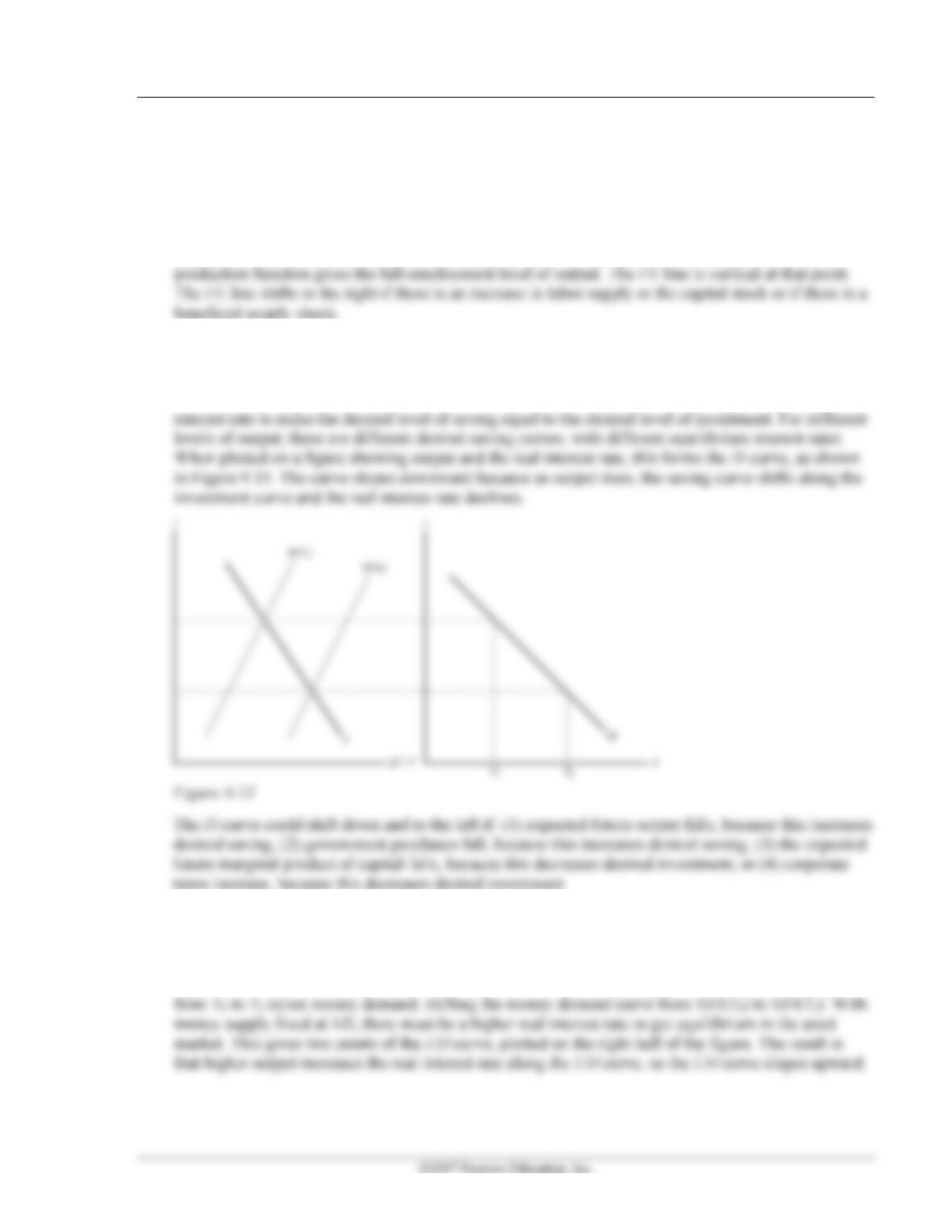
2. The IS curve shows combinations of the real interest rate (r) and output (Y) that leave the goods
market in equilibrium. Equilibrium in the goods market occurs when the aggregate supply of goods
(Y) equals the aggregate demand for goods (Cd + Id + G). Since desired national saving (Sd) is
Y − Cd − G, an equivalent condition is Sd = Id. Equilibrium is achieved by the adjustment of the real
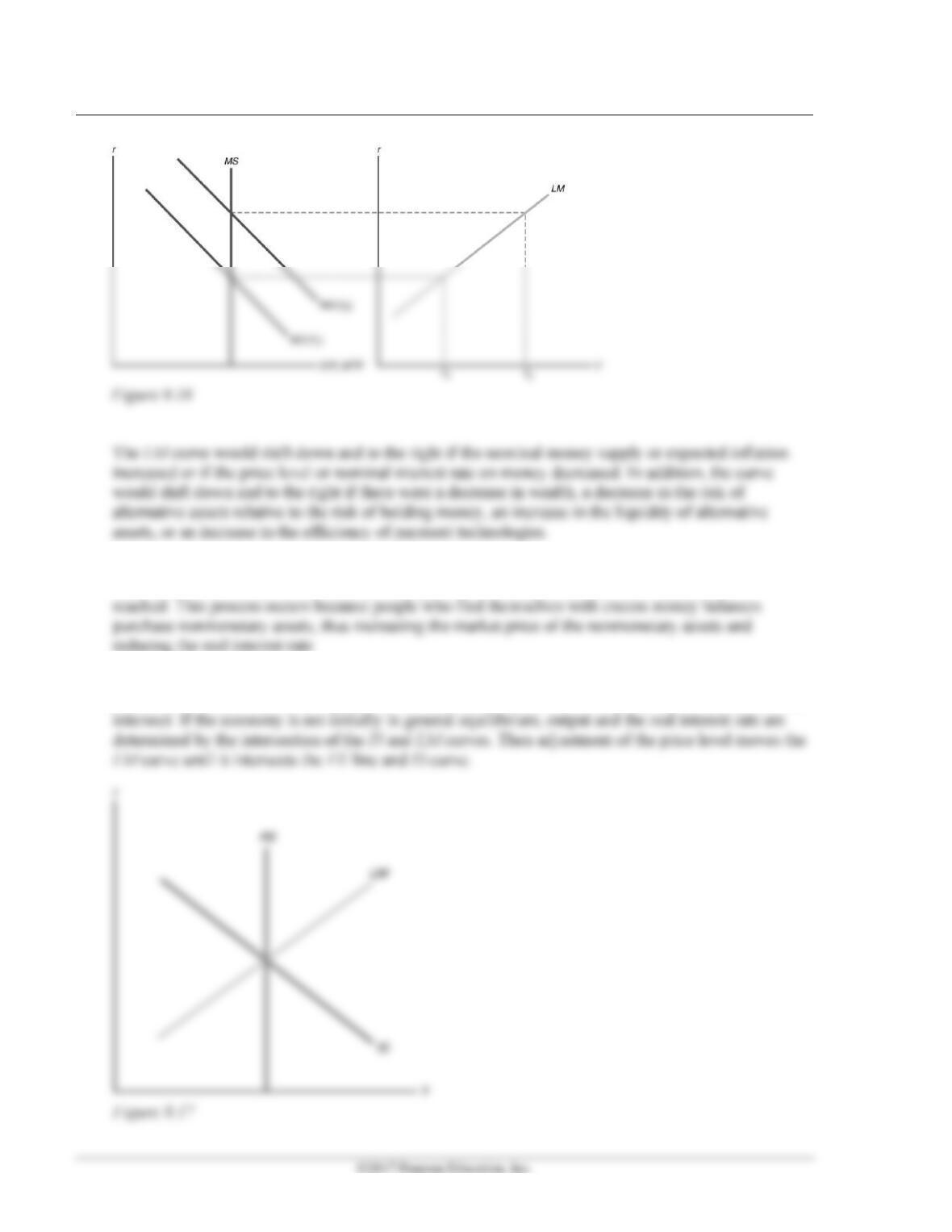
3. The LM curve shows the combinations of output and the real interest rate that maintain equilibrium in
the asset market. Equilibrium in the asset market occurs when real money demand equals the real
money supply.
Figure 9.16 shows the derivation of the LM curve and why it slopes upward. An increase in output
196 Abel/Bernanke/Croushore • Macroeconomics, Ninth Edition
4. For constant output, if real money supply exceeds the real quantity of money demanded, the real
interest rate will decline to increase the real quantity of money demanded until equilibrium is
5. General equilibrium is a situation in which all markets in an economy are simultaneously in
equilibrium. This is shown in Figure 9.17 as the point at which the FE line and the IS and LM curves

Chapter 9 The IS–LM/AD-AS Model: A General Framework for Macroeconomic Analysis 197
6. There is monetary neutrality if a change in the nominal money supply changes the price level but has
no effect on real variables. Once prices adjust, money is neutral in the IS–LM model, because a
7. The aggregate demand curve relates the price level to the aggregate demand for goods and services. It
is downward sloping, because with a fixed nominal money supply, an increase in the price level shifts
the LM curve up, so the level of output at the IS–LM intersection is lower.
Factors that shift the aggregate demand curve up and to the right include (1) an increase in expected
8. The short-run aggregate supply curve is horizontal and the long-run aggregate supply curve is
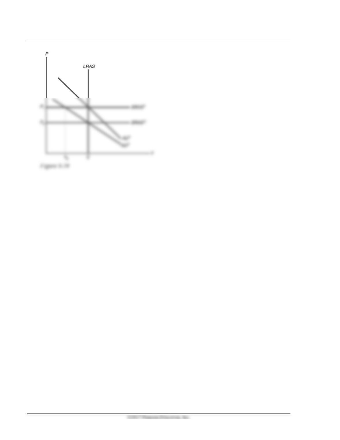
9. In the short run, money is not neutral, but in the long run it is neutral. Suppose the economy is
initially in general equilibrium, as shown in Figure 9.18, where LRAS, SRAS1, and AD1 intersect.
198 Abel/Bernanke/Croushore • Macroeconomics, Ninth Edition
Chapter 9 The IS–LM/AD-AS Model: A General Framework for Macroeconomic Analysis 199
Numerical Problems
1. (a) Sd = Y − Cd − G
= Y − (4000 − 4000r + 0.2Y) − 2000
= −6000 + 4000r + 0.8Y.
(b) (1) Using the equation that goods supplied equals goods demanded gives
So we can use either equilibrium condition to get the same result.
When Y = 10,000,
(c) When G = 2400, desired saving becomes Sd = −6400 + 4000r + 0.8Y. Sd is now 400 less for any
given r and Y.
Similarly, using the equation that goods supplied equals goods demanded gives:
200 Abel/Bernanke/Croushore • Macroeconomics, Ninth Edition
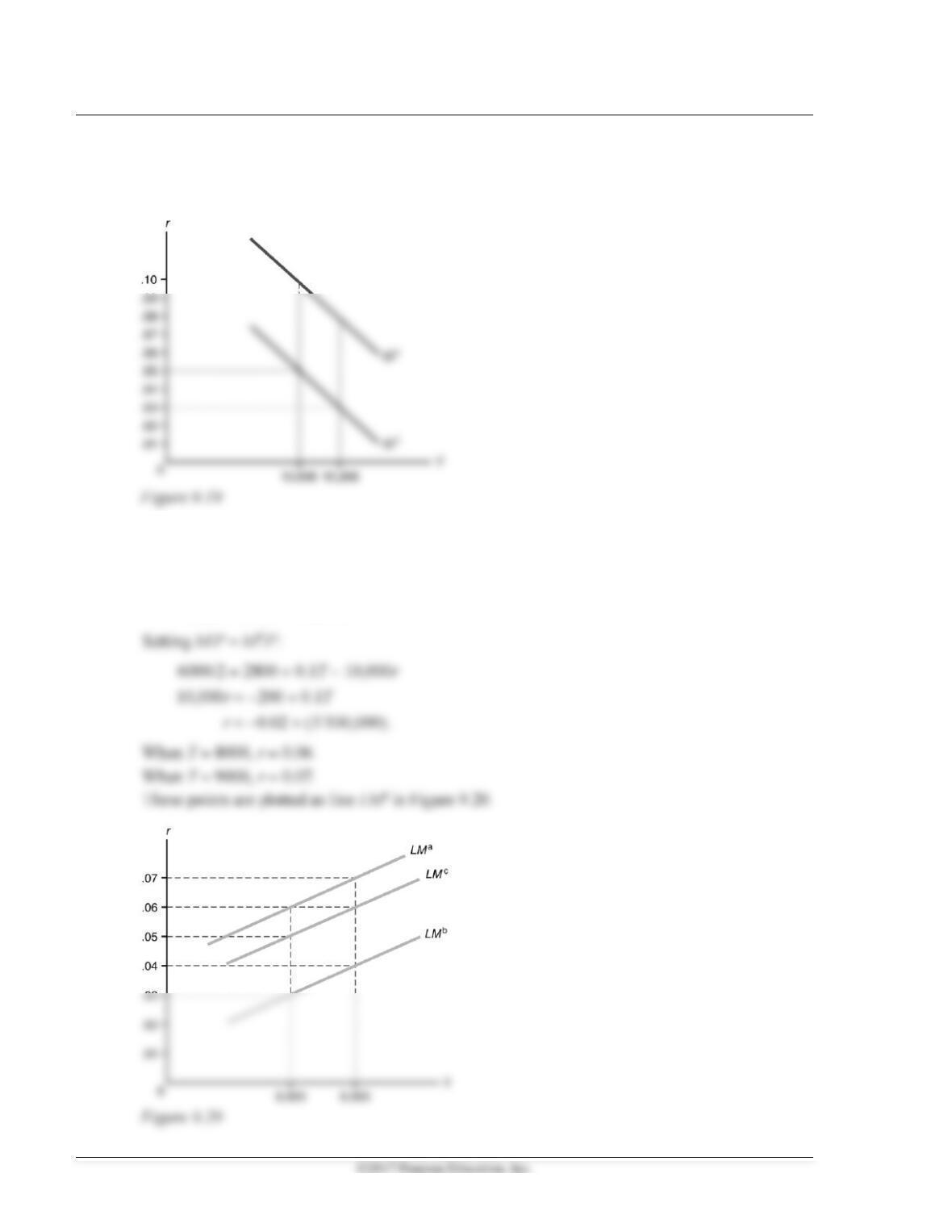
At Y = 10,000, this is 8000r = 8800 − (0.8 10,000) = 800, so r = 0.10. The market-clearing real
interest rate increases from 0.05 to 0.10. Thus the IS curve shifts up and to the right from IS1 to
IS2 in Figure 9.19.
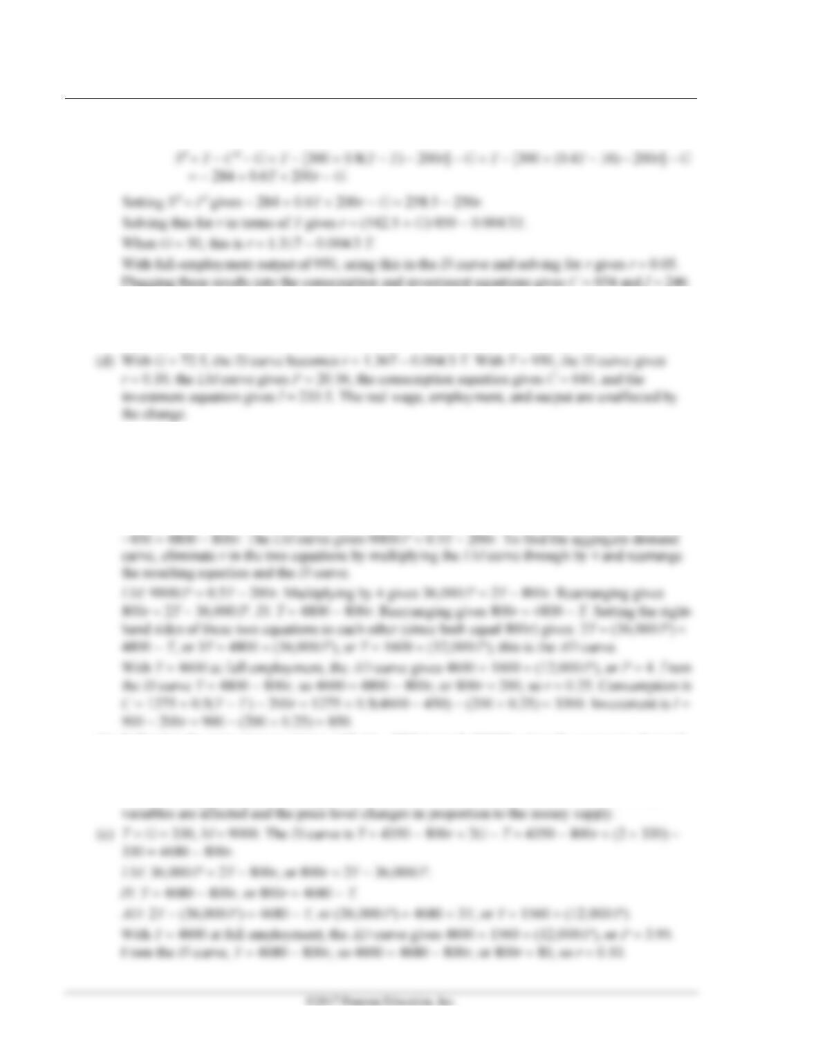
2. (a) Md/P = 3000 + 0.1Y − 10,000i
= 3000 + 0.1Y – 10,000(r +
e)
= 3000 + 0.1Y – 10,000(r + .02)
= 2800 + 0.1Y – 10,000r.

Chapter 9 The IS–LM/AD-AS Model: A General Framework for Macroeconomic Analysis 201
(b) M = 6600, so M/P = 3300. Setting money supply equal to money demand:
(c) Md/P = 3000 + 0.1Y − 10,000(r +
e)
= 3000 + 0.1Y − 10,000r − (10,000 .03)
= 2700 + 0.1Y − 10,000r.
Setting money supply equal to money demand:
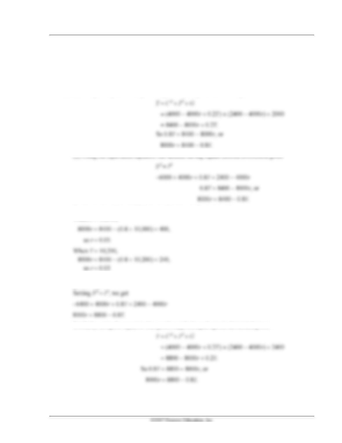
3. (a) First, we’ll find the IS curve.
Sd = Y – Cd – G = Y − [200 + 0.8(Y − T) − 500r] − G = Y − [200 + (0.6Y − 16) − 500r] − G
= −184 + 0.4Y + 500r − G
Setting Sd = Id gives −184 + 0.4Y + 500r − G = 200 − 500r.
4. (a) First, look at labor market equilibrium.
gives w = 9. Using N in the production function gives Y = 950.
202 Abel/Bernanke/Croushore • Macroeconomics, Ninth Edition
(b) Next, look at goods market equilibrium and the IS curve.
Plugging these results into the consumption and investment equations gives C = 654 and I = 246.
(c) Next, look at asset market equilibrium and the LM curve.
Setting money demand equal to money supply gives 9150/P = 0.5Y − 250(r + 0.02), which can be
solved for r = [0.5Y − (5 + 9150/P)]/250. With Y = 950 and r = 0.05, solving for P gives P = 20.
5. The IS curve is found by setting desired saving equal to desired investment. Desired saving is Sd =
Y − Cd − G = Y − [1275 + 0.5(Y − T) − 200r] − G. Setting Sd = Id gives Y − [1275 + 0.5(Y − T) −
200r] − G = 900 − 200r, or Y = 4350 − 800r + 2G − T. The LM curve is M/P = L = 0.5Y − 200i = 0.5Y
− 200(r +
) = 0.5Y − 200r.
(a) T = G = 450, M = 9000. The IS curve gives Y = 4350 − 800r + 2G − T = 4350 − 800r + (2 450)
(b) Following the same steps as above, with M = 4500 instead of 9000, gives the aggregate demand
curve AD: Y = 1600 + (6000/P). With Y = 4600, this gives P = 2. Nothing has changed in the IS
equation, so it still gives r = 0.25. And nothing has changed in either the consumption or
investment equations, so we still get C = 3300 and I = 850. Money is neutral here, as no real

Chapter 9 The IS–LM/AD-AS Model: A General Framework for Macroeconomic Analysis 203
Consumption is C = 1275 + 0.5(Y − T) − 200r = 1275 + 0.5(4600 − 330) − (200 0.10) = 3390.
Investment is I = 900 − 200r = 900 − (200 0.10) = 880.
6. (a) A = 2, f1 = 5, f2 = 0.005, n0 = 55, nw = 10, c0 = 300, cY = 0.8, cr = 200, t0 = 20, t = 0.5, i0 = 258.5,
204 Abel/Bernanke/Croushore • Macroeconomics, Ninth Edition
Analytical Problems
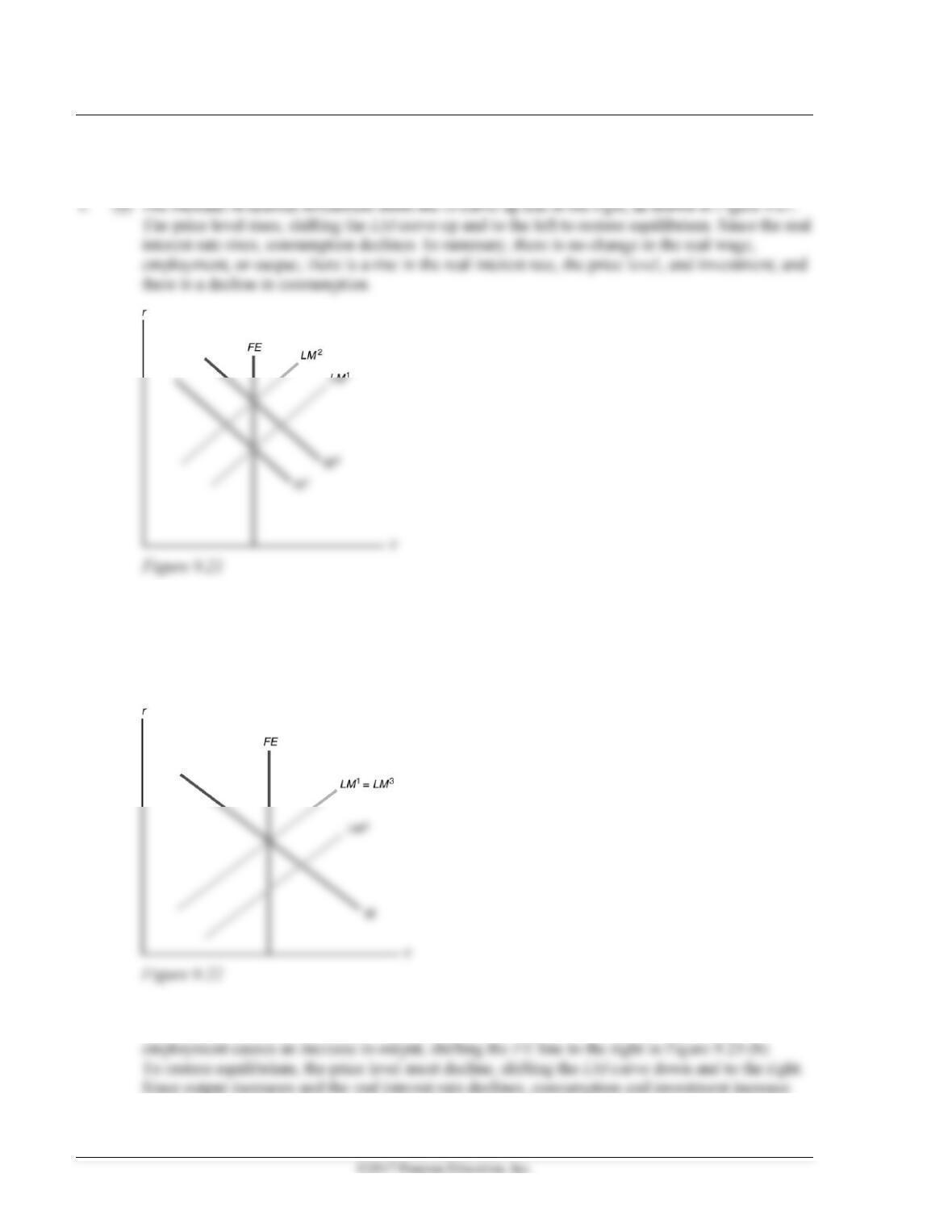
(b) The rise in expected inflation shifts the LM curve down and to the right, as shown in Figure 9.22.
The price level rises, shifting the LM curve up and to the left to restore equilibrium. Since the real
interest rate is unchanged, consumption and investment are unchanged. In summary, there is no
change in the real wage, employment, output, the real interest rate, consumption, or investment;
and there is a rise in the price level.
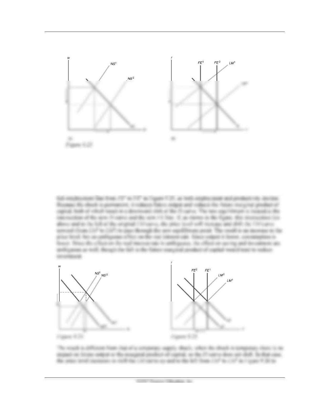
(c) The increase in labor supply is shown as a shift in the labor supply curve in Figure 9.23 (a).
This leads to a decline in the real wage rate and an increase in employment. The rise in
Since output increases and the real interest rate declines, consumption and investment increase.
Chapter 9 The IS–LM/AD-AS Model: A General Framework for Macroeconomic Analysis 205
In summary, the real wage, the real interest rate, and the price level decline; and employment,
output, consumption, and investment rise.
(d) The reduction in the demand for money gives results identical to those in part (b).
2. The increase in the price of oil reduces the marginal product of labor, causing the labor demand curve
to shift to the left from ND1 to ND2 in Figure 9.24. Since households’ expected future incomes decline,
labor supply increases, shifting the labor supply curve from NS1 to NS2 (but by assumption, the shift
to the left in labor demand is larger than the shift to the right in labor supply). At equilibrium, there is
a reduced real wage and lower employment. The productivity shock results in a shift to the left of the
206 Abel/Bernanke/Croushore • Macroeconomics, Ninth Edition
restore equilibrium. In that case, the real interest rate unambiguously increases. Under a permanent
shock, the IS curve shifts down and to the left, so the rise in the real interest rate is less than in the
case of a temporary shock, and the real interest rate can even decline.
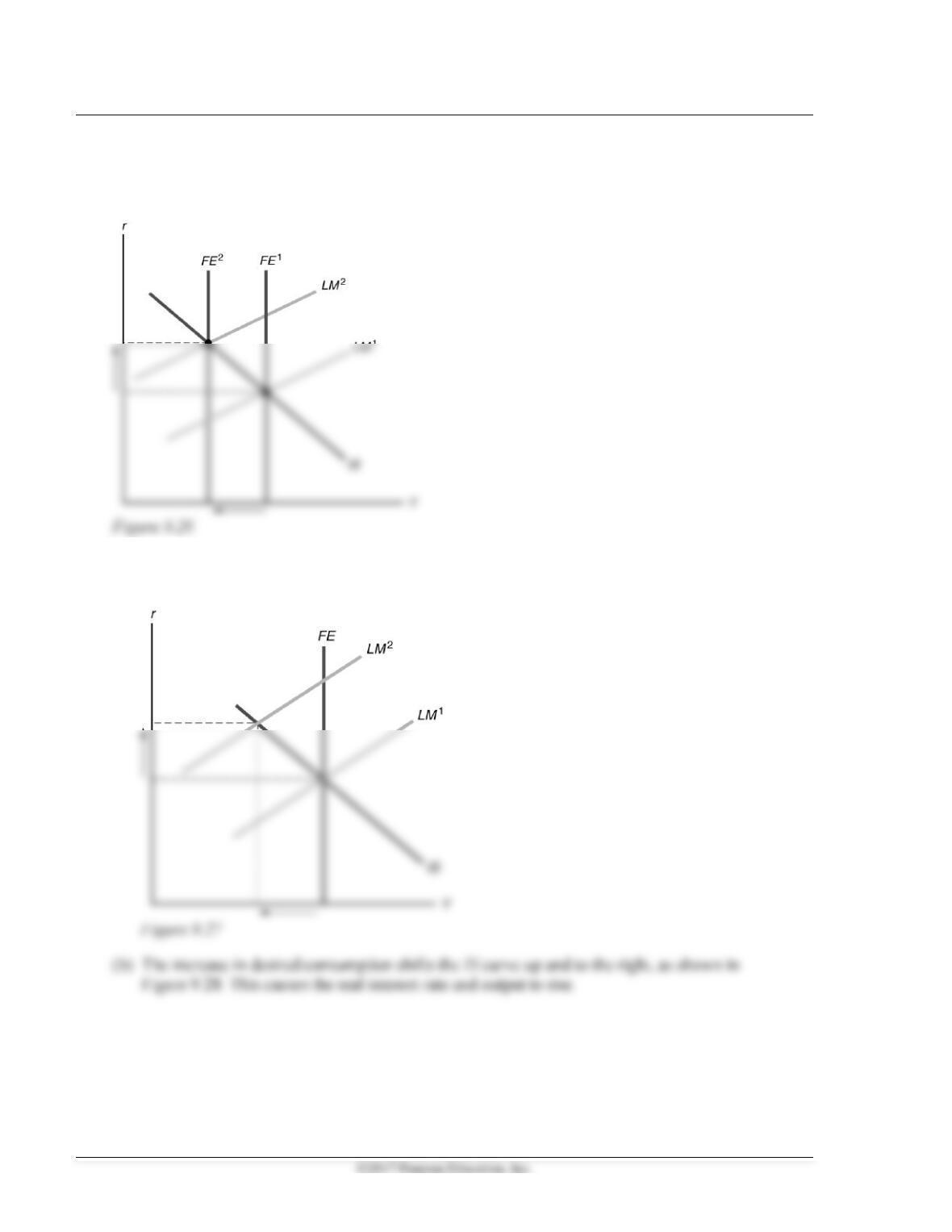
3. (a) The decrease in expected inflation increases real money demand, shifting the LM curve up, as
shown in Figure 9.27. The real interest rate rises and output declines.
Chapter 9 The IS–LM/AD-AS Model: A General Framework for Macroeconomic Analysis 207
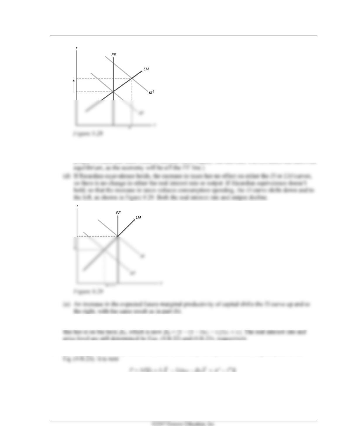
(c) The increase in government purchases shifts the IS curve up and to the right, with the same result
as in part (b). (The FE line also shifts, as the increase in government expenditures reduces
people’s wealth and leads them to increase labor supply, but this shift will not affect the short-run
4. The change in Eq. (9.B.10) has no effect on employment, the real wage, or output. The only effect
5. The change in the money demand function affects only the equation determining the price level,
Y
IS
Y