
103
CHAPTER 9
TEACHING NOTES
The coverage of RESET in this chapter recognizes that it is a test for neglected nonlinearities,
The Davidson-MacKinnon test can be useful for detecting functional form misspecification,
especially when one has in mind a specific alternative, nonnested model. It has the advantage of
always being a one degree of freedom test.
I think the proxy variable material is important, but the main points can be made with Examples
The short section on random coefficient models is intended as a simple introduction to the idea;
it is not needed for any other parts of the book.
I rarely get to teach the measurement error material in a first-semester course, although the
The result on exogenous sample selection is easy to discuss, with more details given in Chapter
17. The effects of outliers can be illustrated using the examples. I think the infant mortality

104
SOLUTIONS TO PROBLEMS
9.1 There is functional form misspecification if
6
0 or
7
0, where these are the population
9.2 [Instructor’s Note: Out of the 186 records in VOTE2.RAW, three have voteA88 less than 50,
which means the incumbent running in 1990 cannot be the candidate who received voteA88
percent of the vote in 1988. You might want to reestimate the equation dropping these three
observations.]
(i) The coefficient on voteA88 implies that if candidate A had one more percentage point of
(ii) Naturally, the coefficients change, but not in important ways, especially once statistical
9.3 (i) Eligibility for the federally funded school lunch program is very tightly linked to being
economically disadvantaged. Therefore, the percentage of students eligible for the lunch program
is very similar to the percentage of students living in poverty.
(ii) We can use our usual reasoning on omitting important variables from a regression
equation. The variables log(expend) and lnchprg are negatively correlated: school districts with

(iv) Both math10 and lnchprg are percentages. Therefore, a ten percentage point increase in
lnchprg leads to about a 3.23 percentage point fall in math10, a sizeable effect.
(v) In column (1) we are explaining very little of the variation in pass rates on the MEAP
9.4 (i) For the CEV assumptions to hold, we must be able to write tvhours = tvhours* + e0,
where the measurement error e0 has zero mean and is uncorrelated with tvhours* and each
explanatory variable in the equation. (Note that for OLS to consistently estimate the parameters
we do not need e0 to be uncorrelated with tvhours*.)
(ii) The CEV assumptions are unlikely to hold in this example. For children who do not
9.5 The sample selection in this case is arguably endogenous. Because prospective students may
look at campus crime as one factor in deciding where to attend college, colleges with high crime
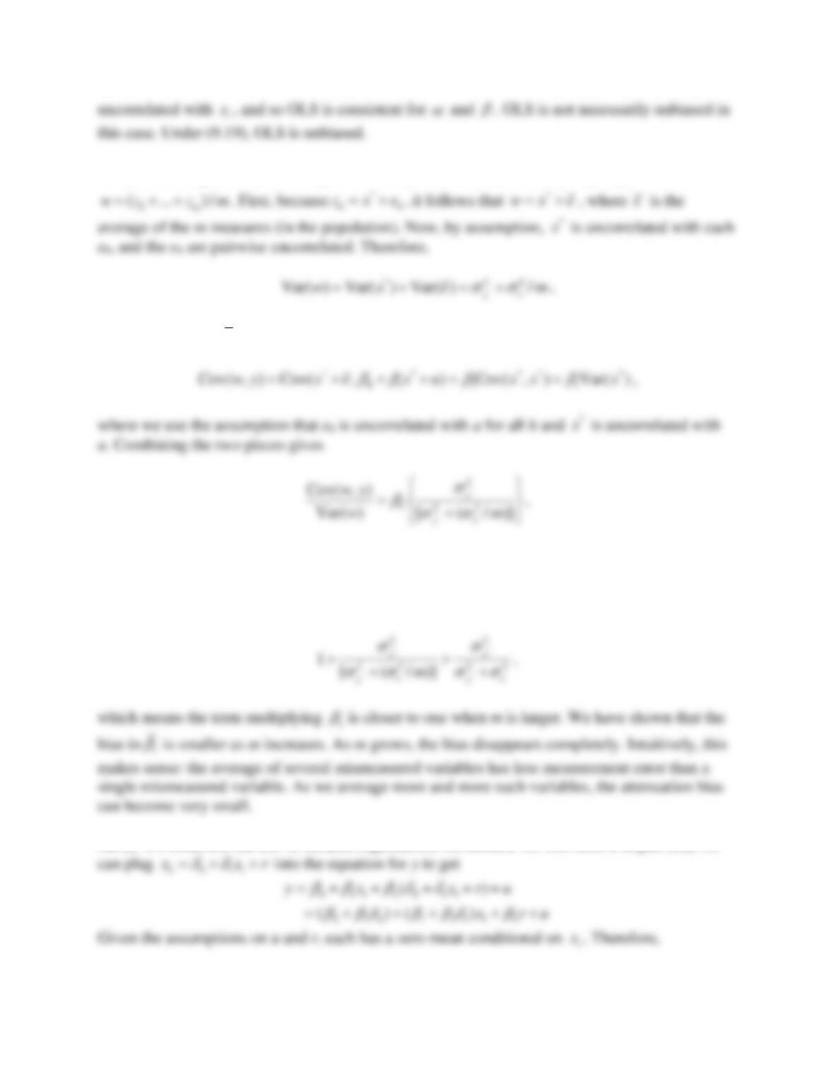
9.6 Following the hint, we write
iii uxy ++=
where
iiii xdcu +=
and
−= ii ac
and
−= ii bd
. Now,
E( ) 0
i
c=
and
E( ) Cov( , )
i i i i
d x b x=
106
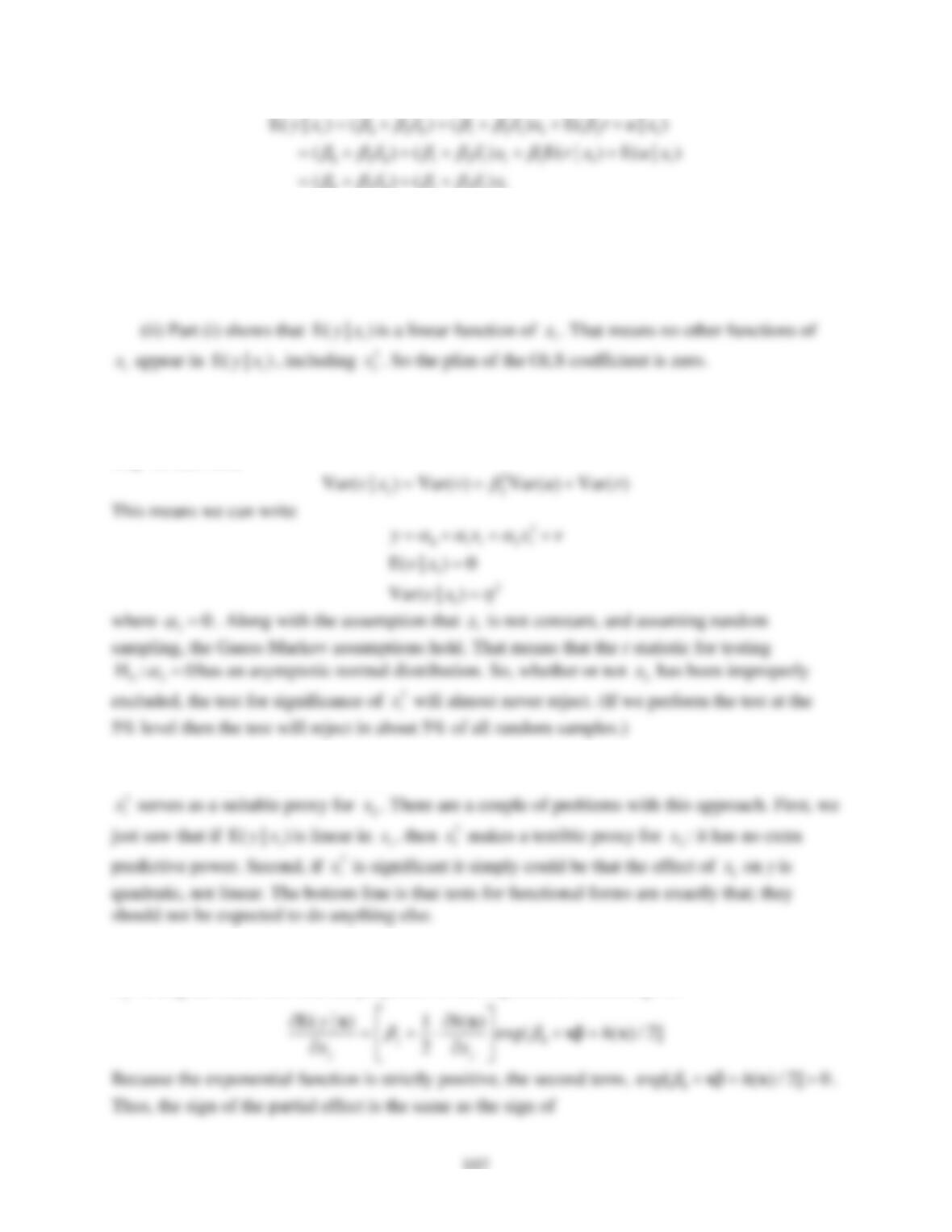
9.7 (i) Following the hint, we compute
Cov( , )wy
and
Var( )w
, where
*
01
y x u
= + +
and
where we use
2
Var( ) /
e
em
=
. Next,
which is what we wanted to show.
(ii) Because
22
/
ee
m
for all m > 1,
*
22
( / )
e
xm
+
<
*
22
e
x
+
for all m > 1. Therefore
9.8 (i) We could use the law of iterated expectations or, because we will need it in part (iii), we
107
0 2 0 1 2 1 1
Given random sampling we can read the probability limits from regressing y on x from the
conditional expectation. The plim of the slope coefficient is
1 2 1
+
. Unless
20
=
or
10
=
the simple regression estimator is inconsistent for
1
1
x
.
(iii) We already did the substitution in the solution to (i). For completeness, note that the zero
conditional mean assumption on u means that u is uncorrelated with r conditional on
1
x
. This is
why we can write
2
1
x
(iv) The suggesting of adding
2
1
x
to test for omission of another variable,
2
x
, presumes that
2
1
x
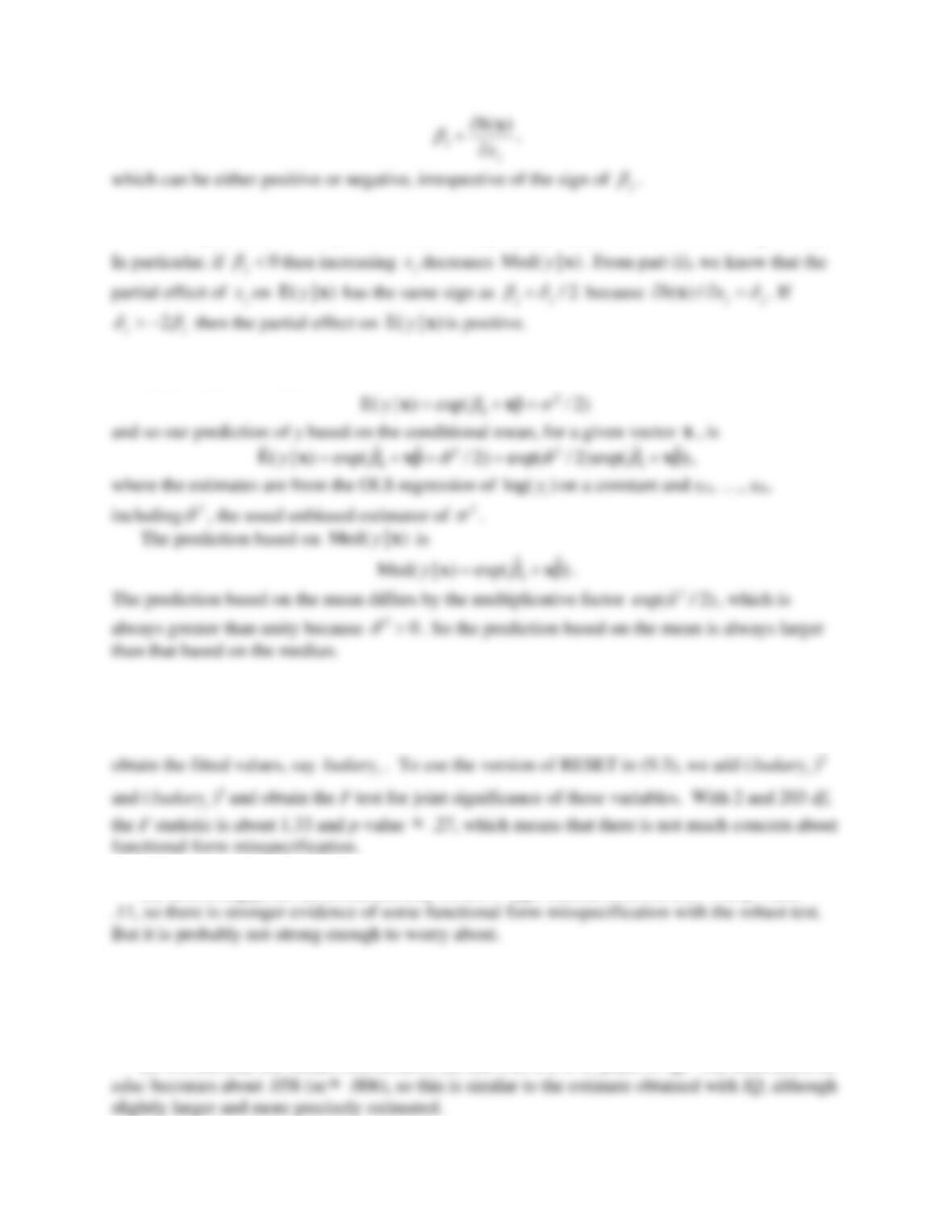
9.9 (i) We can use calculus to find the partial derivative of
E( | )yx
with respect to any element
j
x
. Using the chain rule and the properties of the exponential function gives
108
(ii) The partial effect of
j
x
on
Med( | )yx
is
0
exp( β)
j
+x
, which as the same sign as
j
Med( | )yx
.
(iii) If
2
()h
=x
then
SOLUTIONS TO COMPUTER EXERCISES
C9.1 (i) To obtain the RESET F statistic, we estimate the model in Computer Exercise 7.5 and
(ii) Interestingly, the heteroskedasticity-robust F-type statistic is about 2.24 with p-value
C9.2 [Instructor’s Note: If educ
KWW is used along with KWW, the interaction term is
significant. This is in contrast to when IQ is used as the proxy. You may want to pursue this as
an additional part to the exercise.]
(i) We estimate the model from column (2) but with KWW in place of IQ. The coefficient on
(ii) When KWW and IQ are both used as proxies, the coefficient on educ becomes about .049
(iii) The t statistic on IQ is about 3.08 while that on KWW is about 2.07, so each is significant
C9.3 (i) If the grants were awarded to firms based on firm or worker characteristics, grant could
easily be correlated with such factors that affect productivity. In the simple regression model,
these are contained in u.
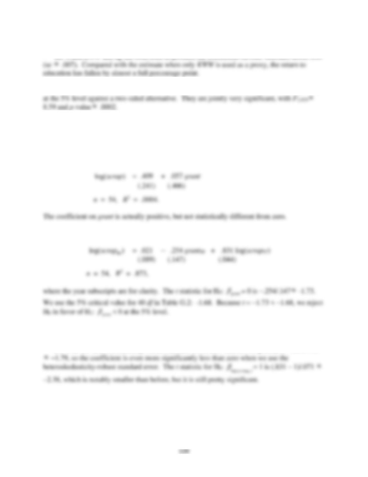
(ii) The simple regression estimates using the 1988 data are
(iii) When we add log(scrap87) to the equation, we obtain
(iv) The t statistic is (.831 – 1)/.044
−3.84, which is a strong rejection of H0.
(v) With the heteroskedasticity-robust standard error, the t statistic for grant88 is −.254/.142
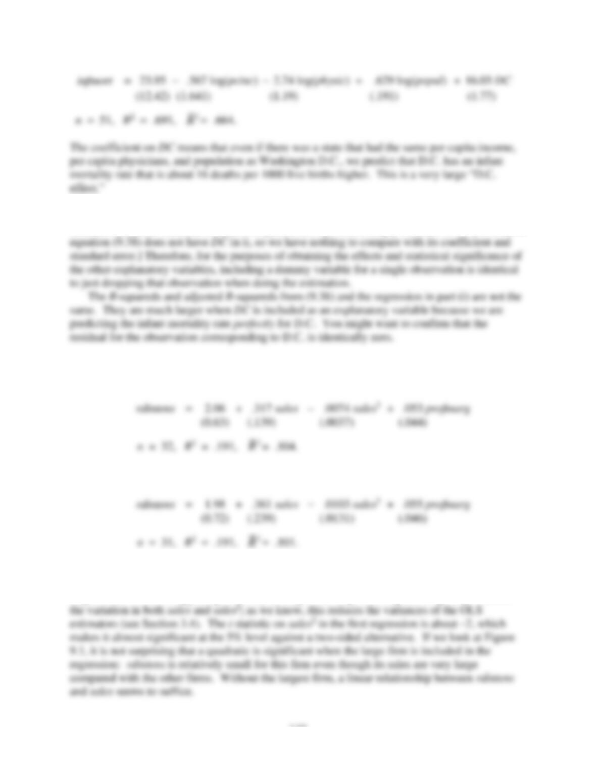
C9.4 (i) Adding DC to the regression in equation (9.37) gives
110
(ii) In the regression from part (i), the intercept and all slope coefficients, along with their
standard errors, are identical to those in equation (9.38), which simply excludes D.C. [Of course,
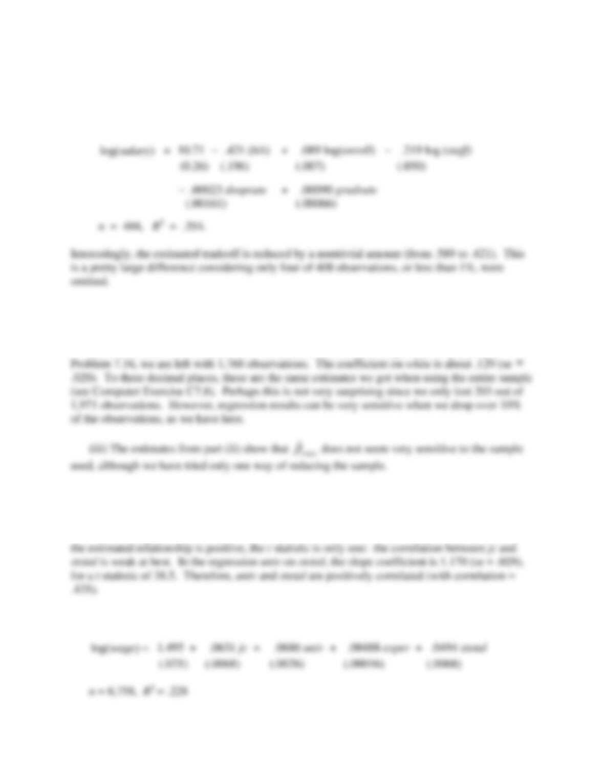
C9.5 With sales defined to be in billions of dollars, we obtain the following estimated equation
using all companies in the sample:
When we drop the largest company (with sales of roughly $39.7 billion), we obtain
When the largest company is left in the sample, the quadratic term is statistically significant,
even though the coefficient on the quadratic is less in absolute value than when we drop the
largest firm. What is happening is that by leaving in the large sales figure, we greatly increase
111
C9.6 (i) Only four of the 408 schools have b/s less than .01.
(ii) We estimate the model in column (3) of Table 4.3, omitting schools with b/s < .01:
C9.7 (i) 205 observations out of the 1,989 records in the sample have obrate > 40. (Data are
missing for some variables, so not all of the 1,989 observations are used in the regressions.)
(ii) When observations with obrat > 40 are excluded from the regression in part (iii) of
C9.8 (i) The mean of stotal is .047, its standard deviation is .854, the minimum value is –3.32,
and the maximum value is 2.24.
(ii) In the regression jc on stotal, the slope coefficient is .011 (se = .011). Therefore, while
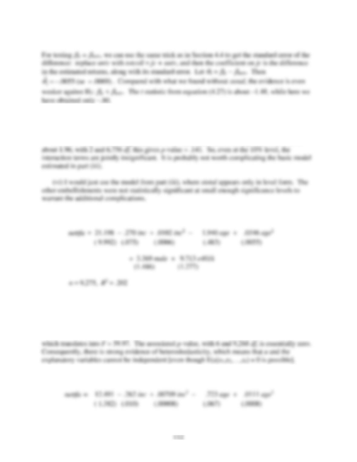
(iii) When we add stotal to (4.17) and estimate the resulting equation by OLS, we get
(iv) When stotal2 is added to the equation, its coefficient is .0019 (t statistic = .40).
Therefore, there is no reason to add the quadratic term.
(v) The F statistic for testing exclusion of the interaction terms stotaljc and stotaluniv is
C9.9 (i) The equation estimated by OLS is
The coefficient on e401k means that, holding other things in the equation fixed, the average level
of net financial assets is about $9,713 higher for a family eligible for a 401(k) than for a family
not eligible.
(ii) The OLS regression of
2
ˆi
u
on inci,
2
i
inc
, agei,
2
i
age
, malei, and e401ki gives
2
2
ˆ
u
R=
.0374,
(iii) The equation estimated by LAD is

113
(iv) The findings from parts (i) and (iii) are not in conflict. We are finding that 401(k)
C9.10 (i) About .416 of the mean receive training in JTRAIN2, whereas only .069 receive
(ii) The simple regression gives
(iii) Adding all of the control listed changes the coefficient on train to 1.68 (se = .63). This
(iv) The simple regression coefficient on train is −15.20 (se = 1.15). This implies a huge

114
(v) For JTRAIN2, the average is 1.74, the standard deviation is 3.90, the minimum is 0, and
(vi) For JTRAIN2, which uses 427 observations, the estimate on train is similar to before,
(viii) When we base our analysis on comparable samples – roughly representative of the
C9.11 (i) The regression gives
ˆexec
= .085 with t = .30. The positive coefficient means that there
is no deterrent effect, and the coefficient is not statistically different from zero.
(ii) Texas had 34 executions over the period, which is more than three times the next highest
(iv) When a Texas dummy is added to the regression from part (iii), its t is only −.37 (and the
115
C9.12 (i) The coefficient on bs is about −.52, with usual standard error .110. Using this standard
(ii) Dropping the four observations with bs > .5 gives
ˆbs
= −.186 with (robust) t = −1.27.
The practical significance of the coefficient is much lower, and it is no longer statistically
different from zero.
(iii) One can verify that “dummying out” the four observations does give the same estimates
(iv) The coefficient on bs with only observation 1,508 dropped is about −.20, which is a big
(v) The findings in part (iv) show that, if an observation is extreme enough, it can exert much
(vi) The LAD estimate of
bs
using the full sample is about −.109 (t = −1.01). When
observation 1,508 is dropped, the estimate is −.097 (t = −0.81). The change in the estimate is
modest, and, besides, it is statistically insignificant in both cases.
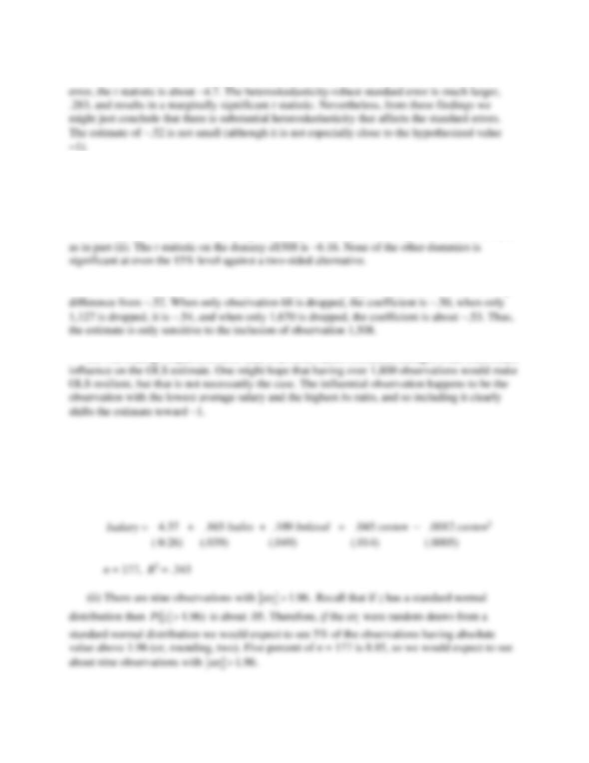
C9.13 (i) The estimated equation, with the usual OLS standard errors in parentheses, is

116
(iii) Here is the estimated equation using only the observations with
1.96
i
str
. Only the
coefficients are reported:
(iv) Using LAD on the entire sample (coefficients only) gives
(v) The previous findings show that it is not always true that LAD estimates will be closer to