CHAPTER 9
Perfect Competition in a Single
Market
A. Summary
This chapter develops the familiar “Marshall Cross” analysis of perfectly
competitive pricing. By assuming that each firm takes market price as given,
the short-run market supply curve is shown to be the horizontal sum of each
firm’s short-run marginal cost curve. This market supply curve then interacts
with market demand to determine equilibrium price and quantity in the short
run.
Long-run supply responses in perfectly competitive markets are the pri-
mary focus of Chapter 9. Emphasis is placed on the free entry assumption
Chapter 9 also provides a number of illustrations of how the competitive
model can be used. Consumer and producer surplus measures are used exten-
sively to determine the welfare consequences of various actions. Special at-
B. Lecture and Discussion Suggestions
The derivation of short-run supply curves in Chapter 9 is relatively simple
and it may be familiar to students from previous economic courses. For that
Chapter 10: Perfect Competition in a Single Market
128
reached the optimal level) need not be shown explicitly as that does involve a
number of diagrams. Instead, one can show a single, long-term equilibrium
and then describe comparative statics analysis solely in a short-run context.
C. Glossary Entries in the Chapter
• Constant Cost Case
• Consumer Surplus
• Deadweight Loss
• Economically Efficient Allocation of Resources
• Equilibrium Price
SOLUTIONS TO CHAPTER 9 PROBLEMS
9.1 a. Set supply equal to demand to find equilibrium price:
QS = 1,000 = QD = 1600 – 600P.
1,000 = 1,600 – 600P.
600 = 600P
P = 1/pound
Chapter 10: Perfect Competition in a Single Market
129
P = 3/pound
d. QS = 0 = –1,000 + 2,000P
1,000 = 2,000P
e. At equilibrium, QD = QS:
–1,000 + 2,000P = 1,600 – 600P
g. Price will rise by less because in c there can be a supply response. The in-
creased demand does not lead only to a price increase, but also an increase in
the quantity supplied.
The graph shows these various equilibria.
9.2 a. Supply = 100,000. In equilibrium,
100,000 160,000 10,000
SD
Q Q P= = = −
or P = 6.
Chapter 10: Perfect Competition in a Single Market
130
b. For any one firm, quantity supplied by other firms is fixed at 99,900. Demand
Curve is
160,000 10,000 99,900 60,100 10,000
d
q P P= − − = −
.
For a single firm, demand is much more elastic:
,
6
10,000 600
100
qP
e= − = −
i
c. If there are 1,000 firms
1,000 200,000 50,000
Si
Q q P= = − +
.
For equilibrium
For any one firm,
160,000 10,000 (199,800 49,950 )
d
q P P= − − +
Demand curve facing the firm is even more elastic than in the fixed supply case
because of the potential supply response by other firms.
Chapter 10: Perfect Competition in a Single Market
131
a. Short run profit maximization requires P = SMC.
P = .01q2 + .4q + 4
b. Industry with 100 firms has supply curve of
For equilibrium, set demand = supply:
4,000 each firm produces 40Qq==
.
For each firm, total revenue is 1440. Short-run total costs are 703. Profits are
737.
9.4 a. If w = 10, STC = q2 + 10q. SMC = 2q + 10 = P. Hence, q = P/2 – 5.
Industry Supply:
b. Here MC = 2q + .002Q. Set = P for profit maximization.
Hence, q = P/2 – .001Q.
Supply for industry as a whole is
9.5 a. In long-run equilibrium, AC = P and MC = P, so AC = MC.
Chapter 10: Perfect Competition in a Single Market
132
.
2
100
.01 1 .02 1or 10,000
100 gallons
q q q
q
q
− + = − =
=
b. In the long-run P = MC P = $1.
9.6 a. LR supply horizontal at P = MC = AC = 10.
b. Q* = 1,500 – 50P* = 1,000. Each firm produces q* = 20, = 0. There are 50
firms.
For the entire industry
50
1
50 500Q q P= = +
e. Q = 2,000 – 50P. If Q = 1,000, P = 20.
9.7 a. With Q = 400, demand curve yields 400 = 1000 – 5P or P = 120.
For supply, 400 = 4P – 80 or P = 120. Hence, P is an equilibrium price. Total
spending on broccoli is 400 120 = 48,000.
Chapter 10: Perfect Competition in a Single Market
133
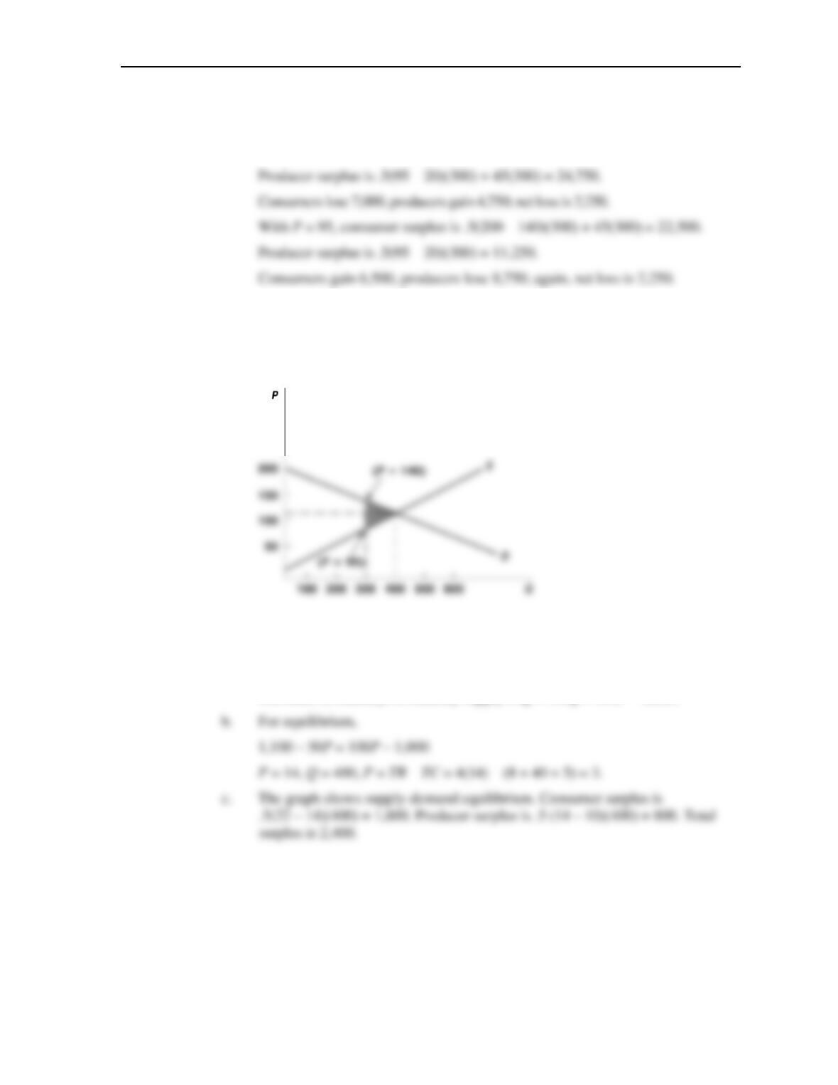
b. With Q = 300, the total loss of surplus would be given by the area of the trian-
gle between the demand and supply curves which is .5(140 – 95)(100) = 2,250.
c. With P = 140, consumer surplus is .5(200 – 140)(300) = 9,000.
d. With Q = 450, demand price would be 110, supply price is 132.50. Total loss
of surplus is .5(132.5 – 110)(5) = 562.50.
Net loss is shared depending where price falls between 110 and 132.5.
e.
9.8 a. For supply, set P = SMC.
P = q + 10
q = P – 10
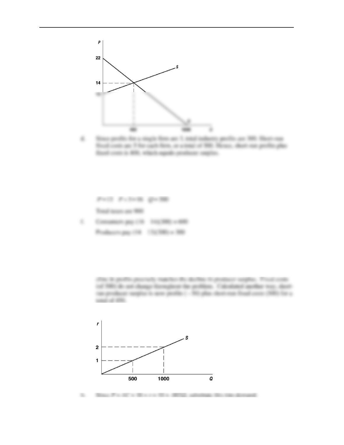
100 firms in industry, so industry supply is Q = 100q = 100P – 1,000.
Chapter 10: Perfect Competition in a Single Market
134
e. New equilibrium is found as:
100 1000 1100 50( 3)Q P P= − = − +
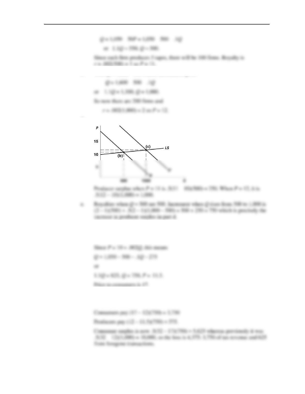
g. Producer surplus is now 0.5(13 – 10)(300) = 450 — a decline of 350 from
problem 11.2c. Now profits for each firm are
(3) 39 39.5 0.5Pq STC− = − = −
Total profits are -50 – a decline from +300 in problem 11.2d. Hence, the de-
9.9 a.
Chapter 10: Perfect Competition in a Single Market
135
c. With Q = 1,600 – 50P, same substitution gives
d.
f. With the tax demand is now
Q = 1,050 – 50(P + 5.5).
g. Total tax collections are
5.5(750) = 4,125.
Chapter 10: Perfect Competition in a Single Market
136
Producer surplus was 1,000; now it is .5(11.5 – 10)(750) = 562.5 a loss of
437.5.
h. All of the lost producer surplus is a loss of royalties. Now
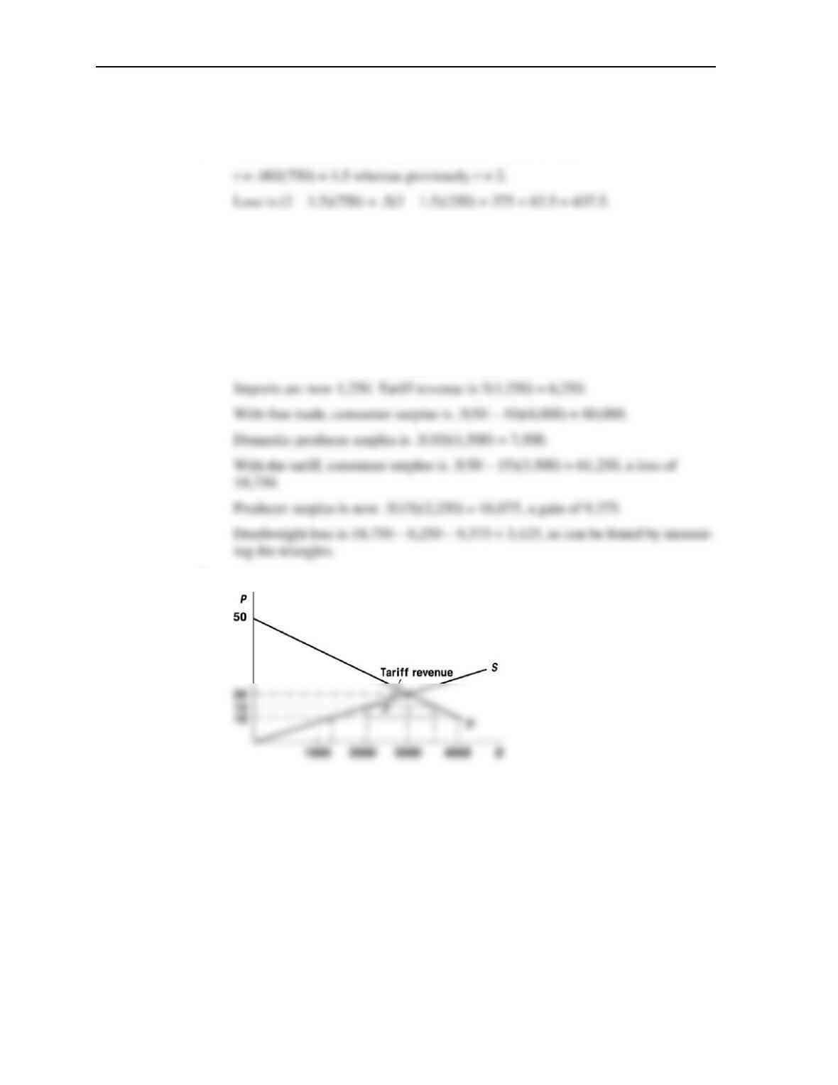
9.10 a. Set quantity supplied equal to quantity demanded
150P = 5,000 – 100P; P = 20, Q = 3,000.
b. P will fall to 10. QD = 4,000, QS = 1,500.
2,500 radios will be imported.
c. Price would now rise to 15. QD = 3,500, QS = 2,250.
d.