CHAPTER 9
AGGREGATE EXPENDITURE AND AGGREGATE DEMAND
In this chapter, you will find:
Learning Outcomes
Chapter Outline with PowerPoint Script
Chapter Summary
Teaching Points (as on Prep Card)
Solutions to Problems Appendix
Experiential Assignments
INTRODUCTION
This chapter is devoted to exploring the individual components of aggregate expenditure—consumption,
investment, government spending, and net exports—as the first elements in developing a theory of
aggregate demand. Consumption is presented as a function of disposable income, and the consumption and
saving functions are connected. Autonomous investment is presented as a function of interest rates and
business expectations. In the body of the chapter, net exports are treated as independent of GDP.
LEARNING OUTCOMES
9-1 Explain what a consumption function illustrates and interpret its slope.
The most predictable and most useful relationship in macroeconomics is between consumption
and income. The more people have available to spend, the more they spend on consumption,
9-2 Describe what can shift the consumption function up or down.
Changes in certain variables, such as household wealth, the price level, interest rates, and consumer
expectations, can shift the consumption function up or down.
9-3 Explain why investment varies more than consumption from year to year.
Investment depends on the market interest rate and on business expectations. Investment fluctuates
Chapter 9 Aggregate Expenditure 124
9-4 Describe how the aggregate expenditure line determines the quantity of aggregate output de-
manded.
The aggregate expenditure line indicates, for a given price level, spending plans at each income level.
9-5 Determine the simple spending multiplier and explain its relevance. The spending multiplier indi-
cates the multiple by which a change in the amount people plan to spend changes real GDP demand-
9-6 Summarize the relationship between the aggregate expenditure line and the aggregate demand
curve.
A higher price level causes a downward shift of the aggregate expenditure line, leading to a lower real
GDP demanded. A lower price level causes an upward shift of the aggregate expenditure line, in-
CHAPTER OUTLINE WITH POWERPOINT SCRIPT
USE POWERPOINT SLIDES 2-5 FOR THE FOLLOWING SECTION
Consumption
A First Look at Consumption and Income
The Consumption Function
USE POWERPOINT SLIDES 6-9 FOR THE FOLLOWING SECTION
Marginal Propensities to Consume and to Save
MPC, MPS, and the Slope of the Consumption and Savings Functions
Chapter 9 Aggregate Expenditure 125
USE POWERPOINT SLIDES 10-15 FOR THE FOLLOWING SECTION
Nonincome Determinants of Consumption: Cause a shift in the consumption function
Net Wealth and Consumption
• Net wealth: The value of all assets that each household owns minus any liabilities.
– A change in net wealth shifts the consumption and saving functions in opposite directions.
The Price Level
• An increase in the price level:
– Causes a downward shift of the consumption function.
USE POWERPOINT SLIDE 15 FOR THE FOLLOWING SECTION
Investment: Gross private domestic investment is spending on:
• New factories, office buildings, malls, and new equipment
USE POWERPOINT SLIDES 16-18 FOR THE FOLLOWING SECTIONS
Investment Demand Curve
Downward-sloping demand curve for investment: an inverse relationship between quantity of investment
demanded and market interest rate.
USE POWERPOINT SLIDES 19-20 FOR THE FOLLOWING SECTION
Nonincome Determinants of Investment
Market Interest Rate
• If the market interest rate increases:
Chapter 9 Aggregate Expenditure 126
– The opportunity cost of investment increases,
Business Expectations: “Animal” spirits of business.
• If business expectations become more pessimistic about profit prospects:
USE POWERPOINT SLIDES 21-22 FOR THE FOLLOWING SECTION
Government
Government Spending: Federal, state, and local government purchases of goods and services.
USE POWERPOINT SLIDE 23 FOR THE FOLLOWING SECTION
Net Taxes
• Transfer payments: Outright grants from governments to households (Social Security, welfare
USE POWERPOINT SLIDES 24-26 FOR THE FOLLOWING SECTION
Net Exports: The value of exports minus imports
Net Exports and Income: Net exports decline as U.S. income increases because:
• U.S. exports are relatively insensitive to the level of U.S. income but depend on foreign incomes.
Nonincome Determinants of Net Exports: Factors assumed constant include:
Chapter 9 Aggregate Expenditure 127
USE POWERPOINT SLIDES 27-28 FOR THE FOLLOWING SECTION
Composition of Aggregate Expenditure
• Consumption’s share of GDP increased from 62 % during the 1960s to 70 % during the most recent
USE POWERPOINT SLIDE 29 FOR THE FOLLOWING SECTION
Aggregate Expenditure and Income: Each dollar of spending translates directly into a dollar of
income. We continue to assume no capital depreciation nor business saving, and net exports are as-
sumed to be autonomous.
The Components of Aggregate Expenditure: AE = C + I + G +(X
−
M)
What If Spending Exceeds Real GDP? For a given price level, there is only one point along the
USE POWERPOINT SLIDES 30-31 FOR THE FOLLOWING SECTION
The Simple Spending Multiplier
An Increase in Spending: As long as spending exceeds output, production will yield more income, which
will generate more spending.
Round One
Chapter 9 Aggregate Expenditure 128
USE POWERPOINT SLIDES 32-37 FOR THE FOLLOWING SECTION
The Aggregate Demand Curve: For each price level, there is a specific aggregate expenditure line,
which yields a unique real GDP demanded. The aggregate demand curve is derived by altering the
CHAPTER SUMMARY
The most predictable and most useful relationship in macroeconomics is between consumption and
income. The more people have to spend, the more they spend on consumption, other things constant.
The consumption function shows the link between consumption and income in the economy. The slope of
the consumption function reflects the marginal propensity to consume, which is the change in consumption
divided by the change in income. The slope of the saving function reflects the marginal propensity to save,
which is the change in saving divided by the change in income.
Government purchases, which exclude transfer payments, averaged a little less than one-fifth of GDP
during the last decade. Government purchases are based on the public choices of elected officials and are
assumed to be autonomous, or independent of the economy’s income level. Net taxes, or taxes minus
transfer payments, are also assumed for now to be unrelated to income.
The aggregate expenditure line indicates, for a given price level, spending plans at each income level. At a
given price level, real GDP demanded is found where the amount that people plan to spend equals the
amount produced.
Chapter 9 Aggregate Expenditure 129
The simple spending multiplier indicates the multiple by which a change in the amount people plan to
spend changes real GDP demanded. The simple spending multiplier developed in this chapter is 1/(1-
MPC). The larger the MPC, the more is spent and the less is saved, so the larger the simple spending
multiplier. This multiplier is called “simple” because only consumption changes with changes in income.
TEACHING POINTS
1. It is important to take time to explain the meaning and significance of consumption. Most students
will be unfamiliar with the technical meaning of the term. Emphasize that consumption is a flow,
2. In talking about the ability of the consumption function to shift up or down, you might emphasize
the fact that this function is drawn against real (disposable) income. Hence, a shift of this function
3. The text uses the income-expenditure model to determine the quantity of aggregate output demand-
ed. That is, the point of intersection between the aggregate expenditure line and the 45-degree
line determines what quantity of GDP will be demanded for the given price level.
4. The role of inventories is crucial to the process of adjustment to equilibrium. Although actual
spending always equals output, differences between actual and planned spending flows manifest
5. When discussing the simple spending multiplier, point out that any spending that shifts the aggre-
gate expenditure line by $X will change equilibrium income by $X/MPS.
6. The key element for students to appreciate is that the aggregate expenditure determined by the in-
come-expenditure model is simply one point on an aggregate demand curve. Because price changes
Chapter 9 Aggregate Expenditure 130
SOLUTIONS TO PROBLEMS APPENDIX
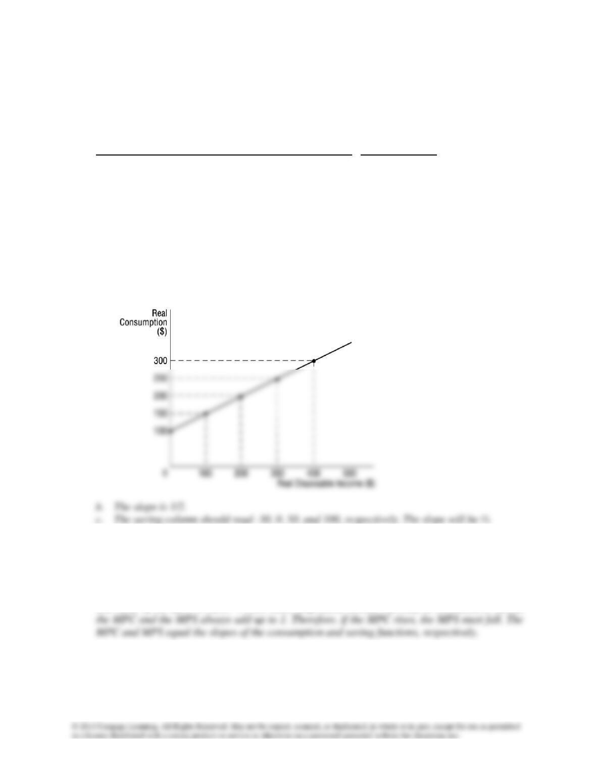
1. (Consumption) Use the following data to answer the questions below.
Real Disposable Consumption
Income (billions) Expenditures (billions) Saving (billions)
$100 $150 $______
200 200 ______
300 250 ______
400 300 ______
a. Graph the consumption function, with consumption spending on the vertical axis and
disposable income on the horizontal axis.
b. If the consumption function is a straight line, what is its slope?
c. Fill in the saving column at each level of income. If the saving function is a straight line,
what is its slope?
a.
2. (MPC and MPS) If consumption increases by $12 billion when real disposable income increases
by $15 billion, what is the value of the MPC? What is the relationship between the MPC and the
MPS? If the MPC increases, what must happen to the MPS? How is the MPC related to the
consumption function? How is the MPS related to the saving function?
The value of the MPC is 12/15 = 0.80. Since disposable income can only be consumed or saved,
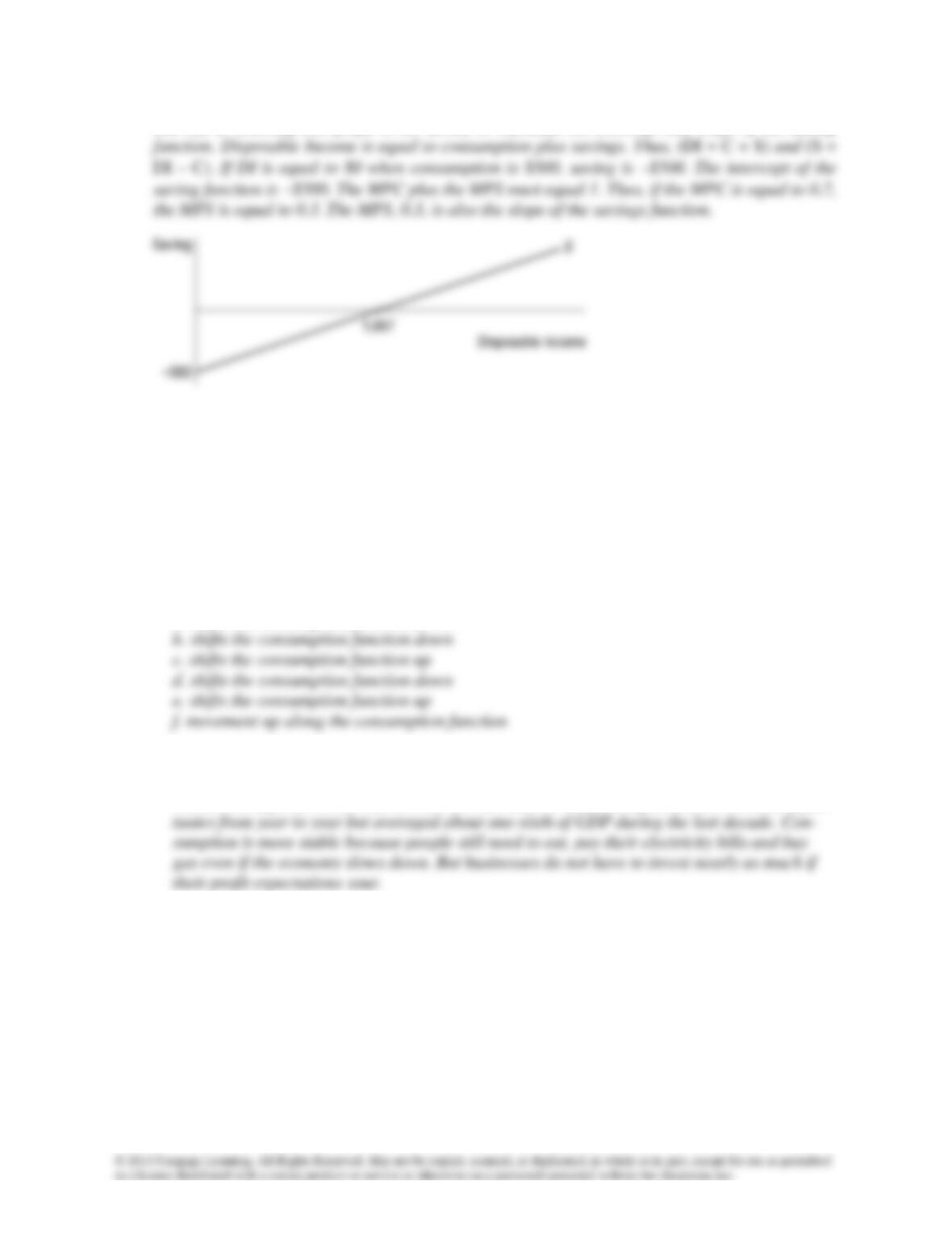
3. (Consumption and Saving) Suppose that consumption equals $500 billion when disposable
income is $0, and that each increase of $100 billion in disposable income causes consumption to
increase by $70 billion. Draw a graph of the saving function using this information.
Chapter 9 Aggregate Expenditure 131
The key to drawing this graph is the ability to calculate the intercept and slope of the saving
4. Consumption Function How would an increase in each of the following affect the consumption
function?
a. Net taxes
b. The interest rate
c. Consumer optimism, or confidence
d. The price level
e. Consumers’ net wealth
f. Disposable income
a. shifts the consumption function down
5. (Investment) Why does investment vary more than consumption from year to year?
Investment depends on the market interest rate and on business expectations. Investment fluc-
6. (Investment) Why would the following investment expenditures increase as the interest rate
declines?
a. Purchases of a new plant and equipment
b. Construction of new housing
c. Increase of inventories
Chapter 9 Aggregate Expenditure 132
a. As interest rates fall, holding revenue from the use of the equipment constant, it becomes
7. (Aggregate Expenditure) What are the components of aggregate expenditure? In the model
developed in this chapter, which components vary with changes in the level of real GDP? What
determines the slope of the aggregate expenditure line?
The components of aggregate expenditure are (a) consumption, (b) investment, (c) government
8. (GDP Demanded) How is the aggregate expenditure line used to identify real GDP demanded
assuming a given price level?
The aggregate expenditure line indicates, for a given price level, spending plans at each in-
9. (Simple Spending Multiplier) For each of the following values for the MPC, determine the size
of the simple spending multiplier and the total change in real GDP demanded following a $10
billion decrease in spending:
a. MPC = 0.9
b. MPC = 0.75
c. MPC = 0.6
10. (Simple Spending Multiplier) Suppose that the MPC = 0.8 and that $14 trillion of real GDP is
currently being demanded. The government wants to increase real GDP demanded to $15
trillion at the given price level. By how much would it have to increase government spending to
achieve this goal?
The simple spending multiplier is 5. If government spending is increased by $200 million, real
11. (Investment and the Multiplier) This chapter assumes that investment is autonomous. What
would happen to the size of the multiplier if investment increases as real GDP increases?
Explain.
Chapter 9 Aggregate Expenditure 133
12. (Shifts in Aggregate Demand) Assume the simple spending multiplier equals 10. Determine the
size and direction of any changes in the aggregate expenditure line, real GDP demanded, and the
aggregate demand curve for each of the following changes in spending:
a. Spending rises by $8 billion at each income level.
b. Spending falls by $5 billion at each income level.
c. Spending rises by $20 billion at each income level.
a. The aggregate expenditure line shifts upward by $8 billion, equilibrium real GDP
Experiential Assignments
1. Expectations and consumer confidence are important in determining fluctuations in aggregate
spending. What is the present status of consumer confidence as measured by the Conference
Board’s index? Students can find the data, with interpretation, at the Conference Board at
2. Business investment spending is an important component of aggregate expenditure. Have students
review the “Business Bulletin” column on the front page of Thursday’s Wall Street Journal. What are
some recent trends in investment spending? Are they likely to increase or decrease aggregate ex-