
Chapter 9
The IS–LM/AD–AS Model: A General
Framework for Macroeconomic Analysis
◼ Learning Objectives
I. Goals of Chapter 9
A. Combine the labor market (Chapter 3), the goods market (Chapter 4), and the asset market
(Chapter 7) into a complete macroeconomic model (for a closed economy)
D. Section goals
1. Describe the factors that explain the full-employment (FE) line (Sec. 9.1)
2. Discuss the factors that affect the IS curve, which represents equilibrium in the goods
market (Sec. 9.2)
II. Notes to Eighth Edition Users
A. We add a new application: “The 2008 Oil Price Shock”

Chapter 9 The IS–LM/AD-AS Model: A General Framework for Macroeconomic Analysis 179
◼ Teaching Notes
I. The FE Line: Equilibrium in the Labor Market (Sec. 9.1)
A. In the discussion of the labor market in Chapter 3, we showed how equilibrium in the labor
market leads to employment at its full-employment level
N
and output at
Y
Y
C. Factors that shift the FE line
1.
Y
is determined by the full-employment level of employment and the current levels of
capital and productivity; any change in these variables shifts the FE line
II. The IS Curve: Equilibrium in the Goods Market (Sec. 9.2)
A. The goods market clears when desired investment equals desired national saving
180 Abel/Bernanke/Croushore • Macroeconomics, Ninth Edition
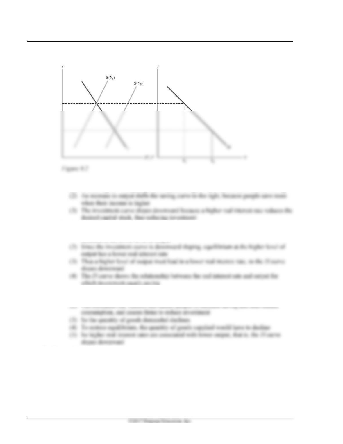
3. Derivation of the IS curve from the saving-investment diagram (Figure 9.2)
a. Key features
(1) The saving curve slopes upward because a higher real interest rate increases saving
b. Consider two different levels of output
(1) At the higher level of output, the saving curve is shifted to the right compared to the
situation at the lower level of output
which investment equals saving
c. Alternative interpretation in terms of goods market equilibrium
(1) Beginning at a point of equilibrium, suppose the real interest rate rises
(2) The increased real interest rate causes people to increase saving and thus reduce
B. Factors that shift the IS curve
1. Any change that reduces desired national saving relative to desired investment shifts the IS
curve up and to the right

Chapter 9 The IS–LM/AD-AS Model: A General Framework for Macroeconomic Analysis 181
a. Intuitively, imagine constant output, so a reduction in saving means more investment
relative to saving; the interest rate must rise to reduce investment and increase saving
(Figure 9.3)
2. Similarly, a change that increases desired national saving relative to desired investment shifts
the IS curve down and to the left
3. An alternative way of stating this is that a change that increases aggregate demand for goods
4. Summary Table 12 lists the factors that shift the IS curve
a. The IS curve shifts up and to the right because of
(1) an increase in expected future output
Numerical Problem 1 asks students to find the IS curve, given equations for consumption and
investment, and looks at how a change in government purchases shifts the curve.
III. The LM Curve: Asset Market Equilibrium (Sec. 9.3)
A. The interest rate and the price of a nonmonetary asset
1. The price of a nonmonetary asset is inversely related to its interest rate or yield
a. Example: A bond pays $10,000 in one year; its current price is $9615, and its interest rate
2. For a given level of expected inflation, the price of a nonmonetary asset is inversely related
to the real interest rate
B. The equality of money demanded and money supplied
182 Abel/Bernanke/Croushore • Macroeconomics, Ninth Edition
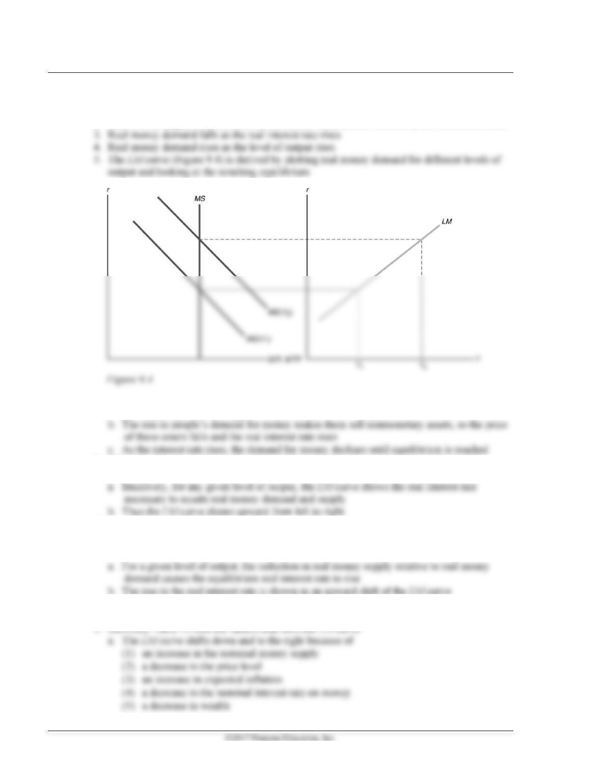
1. Equilibrium in the asset market requires that the real money supply equal the real quantity of
money demanded
2. Real money supply is determined by the central bank and isn’t affect by the real interest rate
6. By what mechanism is equilibrium restored?
a. Starting at equilibrium, suppose output rises, so real money demand increases
7. The LM curve shows the combinations of the real interest rate and output that clear the
asset market
C. Factors that shift the LM curve
1. Any change that reduces real money supply relative to real money demand shifts the LM
curve up
2. Similarly, a change that increases real money supply relative to real money demand shifts the
LM curve down and to the right
Chapter 9 The IS–LM/AD-AS Model: A General Framework for Macroeconomic Analysis 183
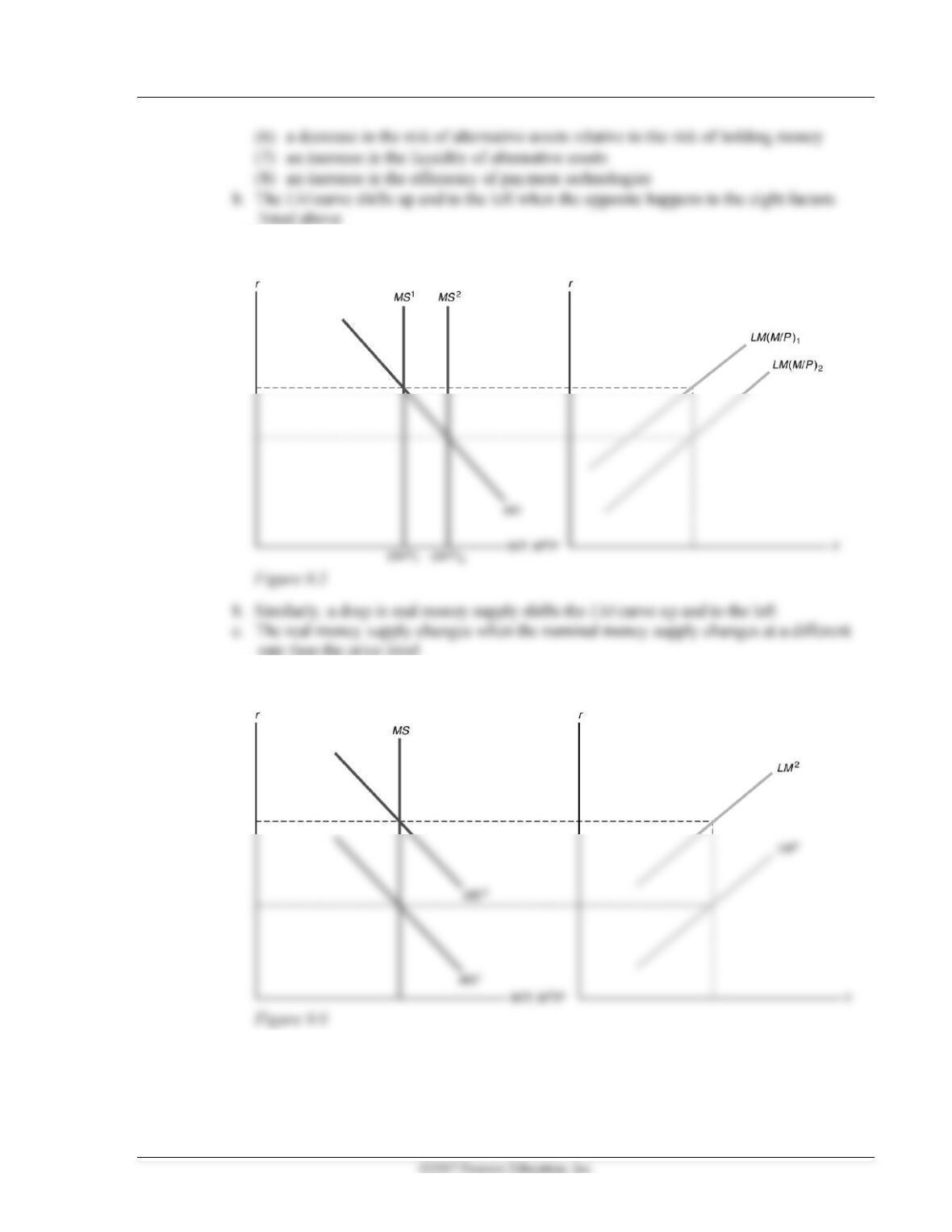
4. Changes in the real money supply
a. An increase in the real money supply shifts the LM curve down and to the right (Figure 9.5)
rate than the price level
5. Changes in real money demand
a. An increase in real money demand shifts the LM curve up and to the left (Figure 9.6)
b. Similarly, a drop in real money demand shifts the LM curve down and to the right

184 Abel/Bernanke/Croushore • Macroeconomics, Ninth Edition
IV. General Equilibrium in the Complete IS–LM Model (Sec. 9.4)
A. When all markets are simultaneously in equilibrium there is a general equilibrium
1. This occurs where the FE, IS, and LM curves intersect (Figure 9.7)
B. Applying the IS–LM framework: A temporary adverse supply shock
1. Suppose the productivity parameter in the production function falls temporarily
2. The supply shock reduces the marginal productivity of labor, hence labor demand
3. There’s no effect of a temporary supply shock on the IS or LM curves
4. Since the FE, IS, and LM curves don’t intersect, the price level adjusts, shifting the LM curve

Chapter 9 The IS–LM/AD-AS Model: A General Framework for Macroeconomic Analysis 185
5. The inflation rate rises temporarily, not permanently
6. Summary: The real wage, employment, and output decline, while the real interest rate and
C. Application: The 2008 oil price shock
1. In 2008, oil prices increased sharply in first half of year
2. In theory, this would make real interest rates increase
Analytical Problem 2 examines the effect on the real interest rate of a permanent oil price shock
compared to a temporary oil price shock.
D. In touch with data and research: Econometric models and macroeconomic forecasts
2. There are three major steps in using an economic model for forecasting
a. An econometric model estimates the parameters of the model (slopes, intercepts,

186 Abel/Bernanke/Croushore • Macroeconomics, Ninth Edition
3. The Federal Reserve Board’s FRB/US model, introduced in 1996, improves on the old model
by better handling of expectations, improved modeling of reactions to shocks, and use of
Theoretical Application
For an overview of the current state of the art in macroeconomic forecasting, see the article by
V. Price Adjustment and the Attainment of General Equilibrium (Sec. 9.5)
A. The effects of a monetary expansion
1. An increase in money supply shifts the LM curve down and to the right
2. Because financial markets respond most quickly to changes in economic conditions, the asset
market responds to the disequilibrium
3. The increase in the money supply causes people to try to get rid of excess money balances by
buying assets, driving the real interest rate down
4. The adjustment of the price level
a. Since the demand for goods exceeds firms’ desired supply of goods, firms raise prices

Chapter 9 The IS–LM/AD-AS Model: A General Framework for Macroeconomic Analysis 187
d. The result is no change in employment, output, or the real interest rate
e. The price level is higher by the same proportion as the increase in the money supply
Numerical Problems 3 and 4 and Analytical Problem 1 look at the complete IS–LM model, including
adjustment of the price level to restore equilibrium.
5. Trend money growth and inflation
d. Often, then, we’ll discuss things in relative terms
(1) The examples can often be thought of as a change in M or P relative to the expected
or trend growth of money and inflation
B. Classical versus Keynesian versions of the IS–LM model
1. There are two key questions in the debate between classical and Keynesian approaches
a. How rapidly does the economy reach general equilibrium?
b. What are the effects of monetary policy on the economy?
2. Price adjustment and the self-correcting economy

188 Abel/Bernanke/Croushore • Macroeconomics, Ninth Edition
(2) If firms change prices instead of output in response to a change in demand, the
adjustment process is almost immediate
d. Keynesian economists see slow adjustment of the price level
3. Monetary neutrality
a. Money is neutral if a change in the nominal money supply changes the price level
proportionately but has no effect on real variables
VI. Aggregate Demand and Aggregate Supply (Sec. 9.6)
A. Use the IS–LM model to develop the AD–AS model
B. The aggregate demand curve
1. The AD curve shows the relationship between the quantity of goods demanded and the price
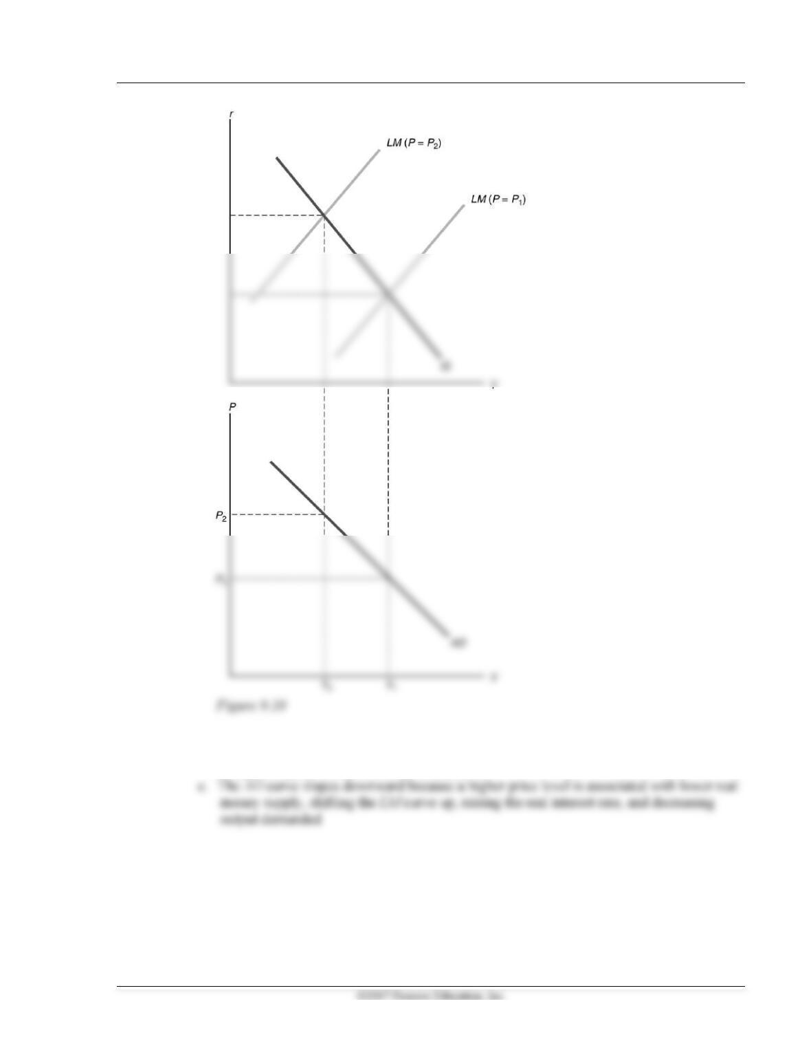
Chapter 9 The IS–LM/AD-AS Model: A General Framework for Macroeconomic Analysis 189
b. The AD curve is unlike other demand curves, which relate the quantity demanded of a
good to its relative price; the AD curve relates the total quantity of goods demanded to
the general price level, not a relative price
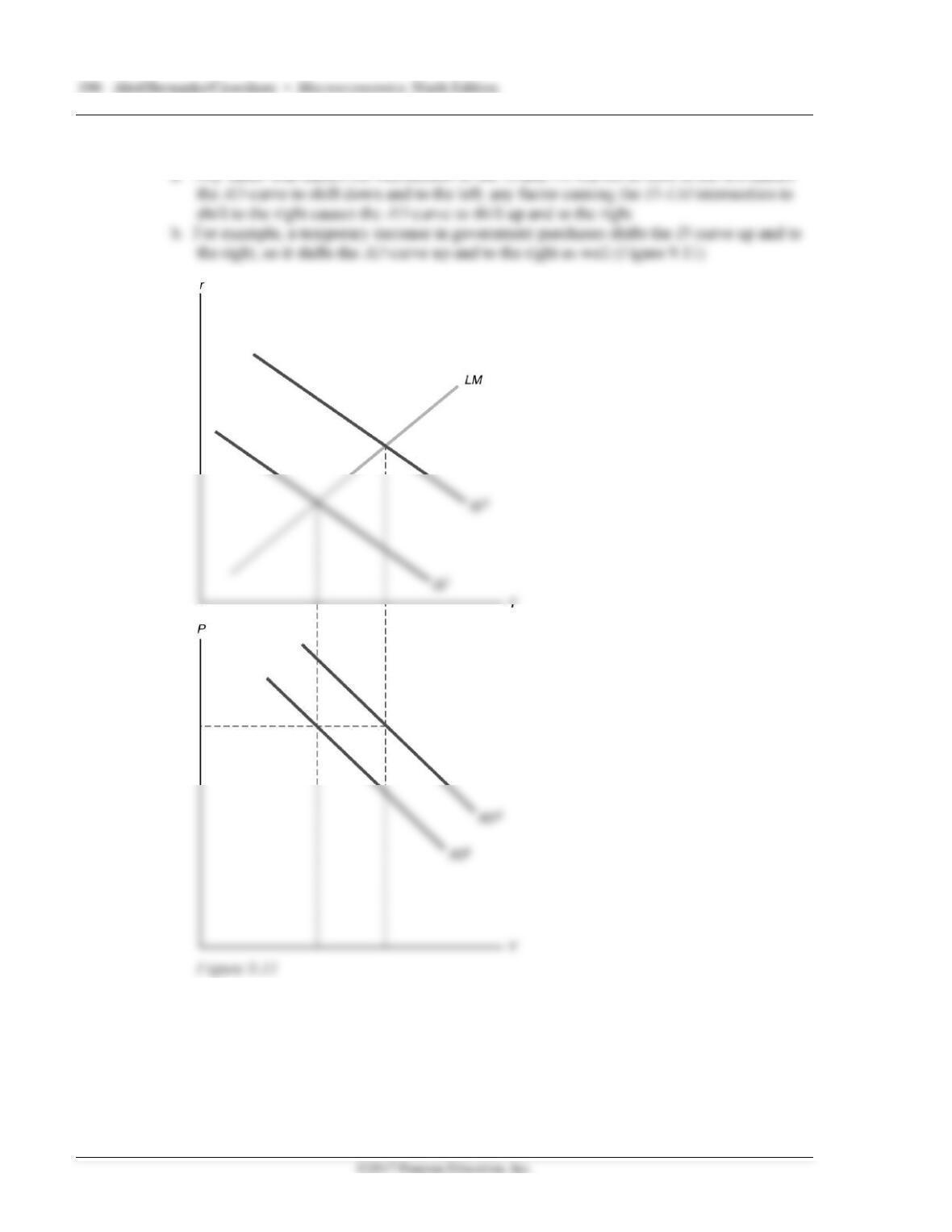
2. Factors that shift the AD curve

Chapter 9 The IS–LM/AD-AS Model: A General Framework for Macroeconomic Analysis 191
(1) Factors that shift the IS curve up and to the right and thus the AD curve up and to the
right as well
)
(2) Factors that shift the LM curve down and to the right and thus the AD curve up and to
the right as well
C. The aggregate supply curve
1. The aggregate supply curve shows the relationship between the price level and the aggregate
amount of output that firms supply
2. In the short run, prices remain fixed, so firms supply whatever output is demanded
3. Full-employment output isn’t affected by the price level, so the long-run aggregate supply
curve (LRAS) is a vertical line at Y =
Y
in Figure 9.12
4. Factors that shift the aggregate supply curves
a. The SRAS curve shifts whenever firms change their prices in the short run
192 Abel/Bernanke/Croushore • Macroeconomics, Ninth Edition
D. Equilibrium in the AD–AS model
1. Short-run equilibrium: AD intersects SRAS
2. Long-run equilibrium: AD intersects LRAS
a. Also called general equilibrium
b. AD, LRAS, and SRAS all intersect at same point (Figure 9.13)
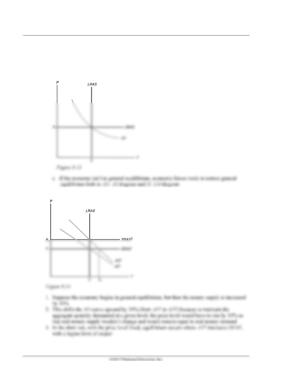
E. Monetary neutrality in the AD–AS model (Figure 9.14 and key diagram 7)