Economics Chapter 9 Homework The Value Obtaining Value Much 198 Greater

Basic Econometrics, Gujarati and Porter

91

CHAPTER 9:

DUMMY VARIABLE REGRESSION MODELS

9.1 (a) If the intercept is present in the model, introduce 11 dummies.

9.2 (a) As per economic theory, the coefficients of X

2

, X

5

are expected

(b) Holding all other factors constant, one would expect that desired

(c) Perhaps, this is due to collinearity between age and education, as

9.3 (a) The relationship between the two variables is expected to be

92

9.4 The results show that the average price was higher by $5.22 per

9.5 (a): Male Professor:

( ) ( )

E Y X

α α β

= + +

(b) Male Professor:

1 2

( ) ( 2 )

i i

E Y X

α α β

= + +

(c) Male Professor

1 2

( ) ( )

i i

E Y X

α α β

= − +

9.6 Following Chapter 8, we can use the t test as follows:

Basic Econometrics, Gujarati and Porter

93

For exactly the same reasoning, to test the hypothesis that the

9.7

(a) & (b):The standard errors of the coefficients of the regression

(9.5.6) can be directly obtained from (9.5.4). But to obtain the

9.8

(a) Neglecting the dummies for the moment, since this is a double

Basic Econometrics, Gujarati and Porter

94

(b) & (c): Since the regressand is in the log form, we have to

dummy coefficients are to be interpreted similarly.

.

9.9

(a) & (c): Ceteris paribus, if the expected inflation rate goes up by 1

percentage point, the average Treasury bill rate (TB) is expected to

go down by about 0.13 percentage point, which does not make

` (b) In late 1979 the then Governor of the Federal Reserve System,

9.10

Write the model as:

Basic Econometrics, Gujarati and Porter

95

9.11

(a) This assignment of the dummy variables assumes a constant

(b) As expected, brand name colas are more expensive than non–

9.12

(a) The coefficient of the income variable in the log form is a semi-

(b) This coefficient shows that the average life expectancy is likely

(c) This regressor is introduced to capture the effect of increasing

(d) The regression equation for countries below the per capita

Basic Econometrics, Gujarati and Porter

equation is:

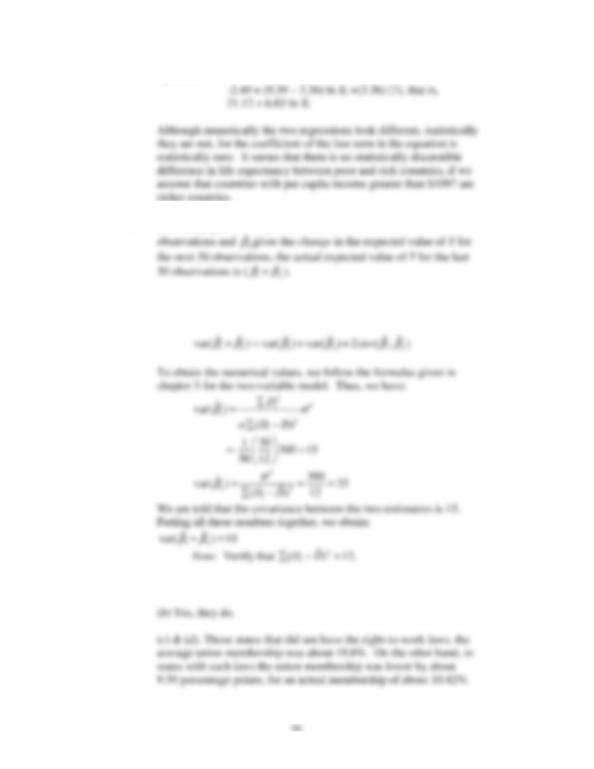
9.13

(a)& (b).

1

β

gives the expected value of Y for the first 20

(c) From the well-known formula to find the sum or difference of

two or more random variables (See App. A), it can be shown that

9.14

(

a

) The expected relationship between the two variables is negative.

97

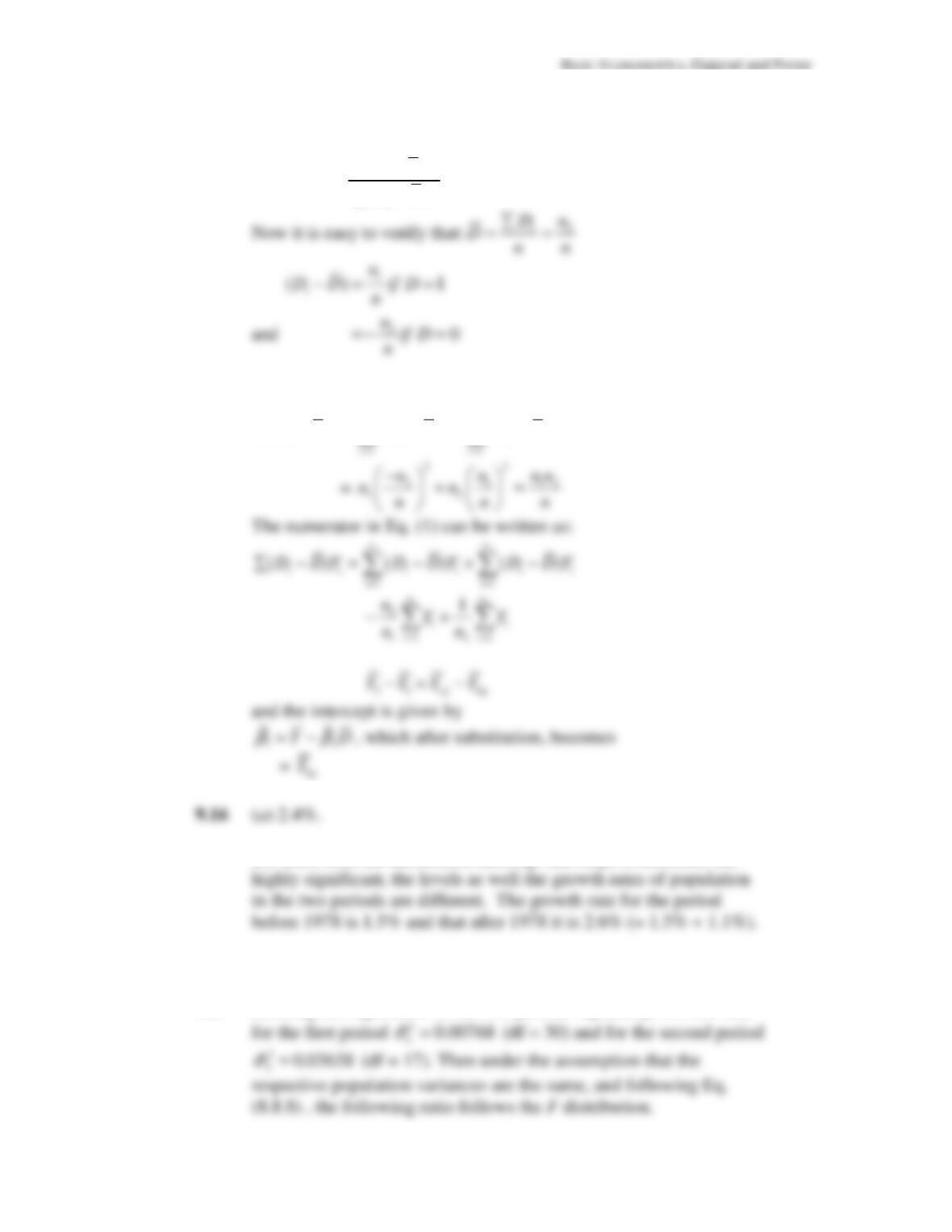
9.15

From the OLS formulas given in Chapter 3, we know that:

2

( )

ˆ

( )

i i

i

D D Y

D D

β

∑−

=∑−

(1)

Now the denominator in Eq. (1) can be written as:

1 2

2 2 2

( ) ( ) ( )

n n

i i i

D D D D D D

∑

− = − + −

∑ ∑

(b) Since both the differential intercept and slope coefficients are

Empirical Exercises

9.17

Running the regression for the two periods separately, we find that

Basic Econometrics, Gujarati and Porter

98

1 2

2

( ),( )

2

1

ˆ

n k n k

F F

σ

− −

=

∼

9.18

Since the dependent variable in models (9.7.3) and (9.7.4) is the

same, we can use the

2

R

version of the F test given in Eq. (8.7.10).

In the present instance, the restricted

2

R

(i.e.,

2

R

) is obtained from

99

9.19

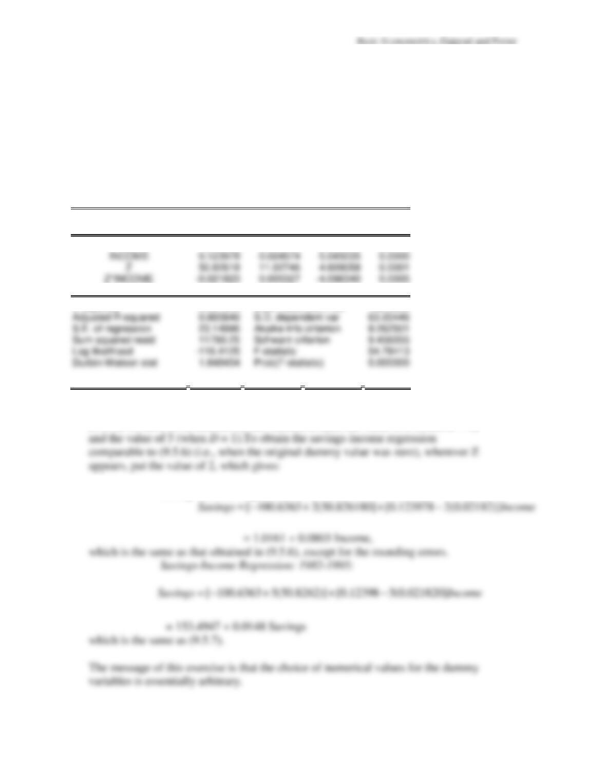
In this case the dummy variable Z takes the value of 2 when D= 0

and it takes the value of 5 when D = 1. Using this dummy

assignment, we get the following regression results:

Dependent Variable: SAVINGS

Method: Least Squares

.

Sample: 1970 1995

Included observations: 26

Variable Coefficient

Std. Error

t-Statistic

Prob.

C -100.6363

37.88404

-2.656429

0.0144

R-squared 0.881944

Mean dependent var 162.0885

Now in comparing the preceding results with those given in (9.5.4), (9.5.6) and

(9.5.7), we have to be careful, for the variable Z takes the value of 2 (when D = 0)

Savings-Income Regression 1970-1981:

100

9.20

As you would suspect, the sign of the dummy coefficient in (9.5.4)

9.21

(

a

) Since the dummy enters in the log form, and since the log of

(

b

) The regression results are as follows (

t

values in parentheses):

Since the dummy coefficient is not statistically significant, for all practical

purposes the two intercept terms are the same. The interpretation of the intercept

It may be interesting to compare the preceding regression results with the following

results, which allow for the interaction effect:

Now you get an entirely different picture, for the differential intercept and slope

9.22

(a) We present the results for the three appliances in the following

tabular form:

Basic Econometrics, Gujarati and Porter

101

Type of Appliance Intercept D

2

D

3

D

4

R

2

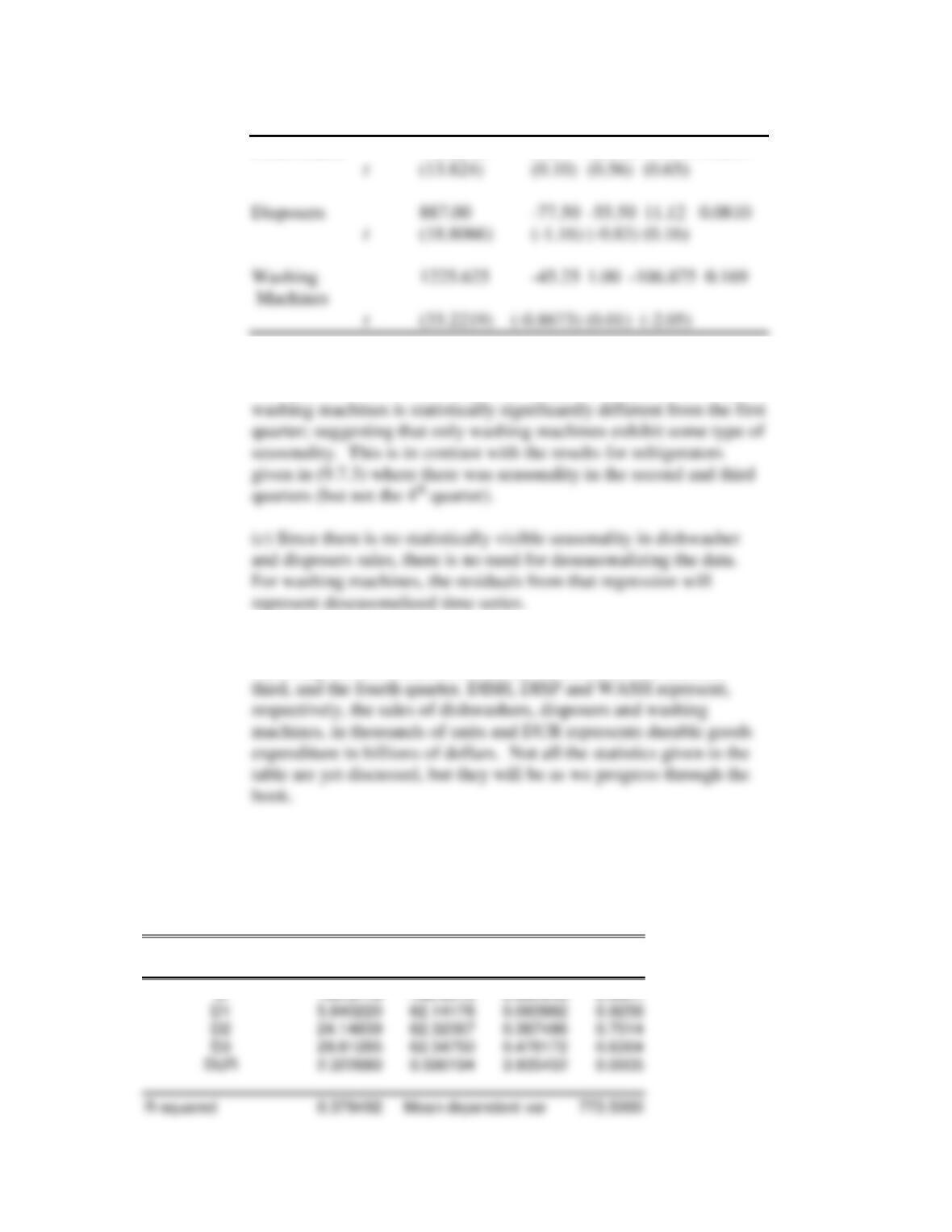
Dishwashers 748.2500 8.25 42.875 49.875 0.0219

(b) The “slope” coefficients are in fact differential intercepts, with

first quarter as the reference quarter. Only the 4

th

quarter dummy for

9.23

The regression results, obtained from EViews are as follows: In the

following table, D

1

, D

2

and D

3

are the dummies for the second,

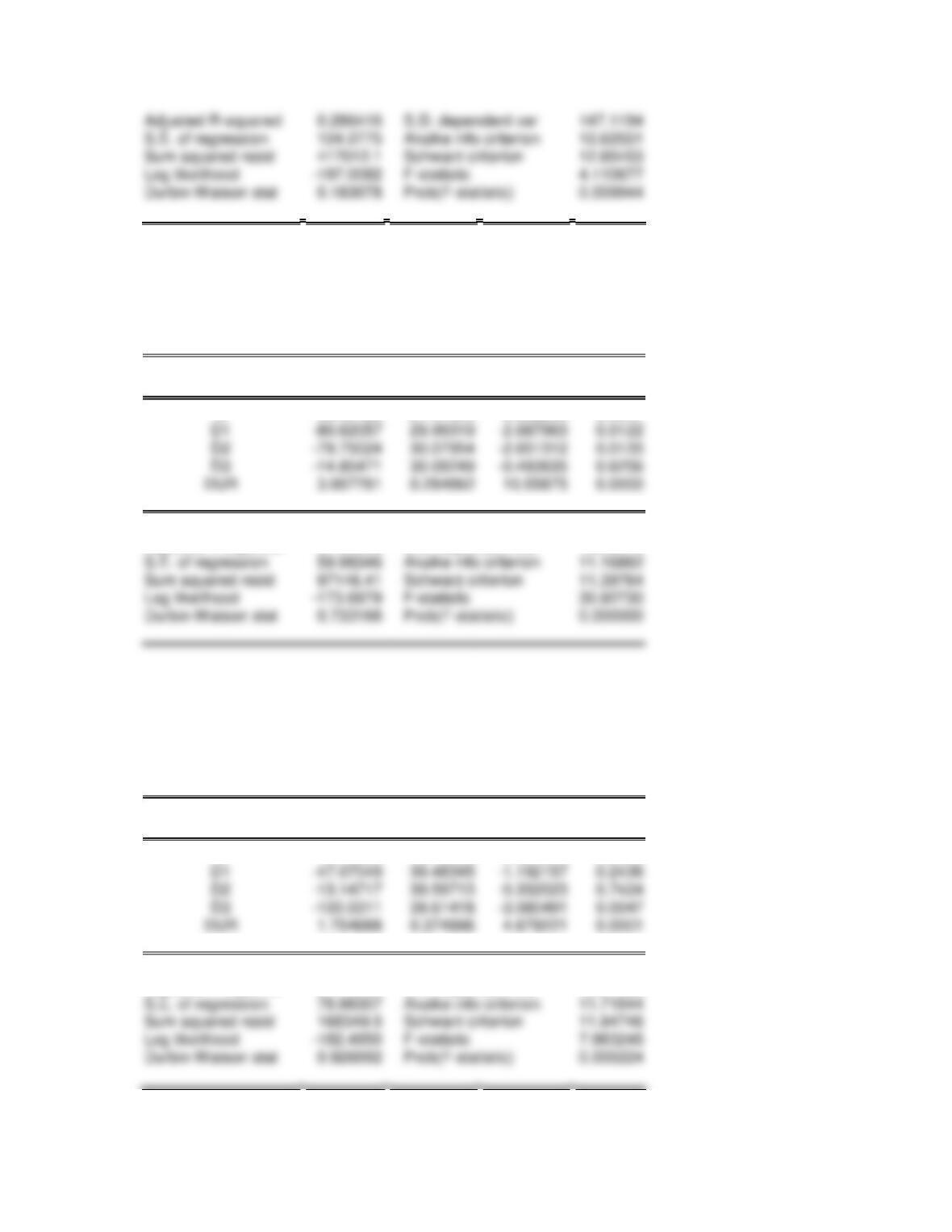
Dependent Variable: DISH

Method: Least Squares

.

Sample: 1978:1 1985:4

Included observations: 32

Variable Coefficient

Std. Error

t-Statistic

Prob.

Basic Econometrics, Gujarati and Porter

102

Dependent Variable: DISP

Method: Least Squares

.

Sample: 1978:1 1985:4

Included observations: 32

Variable Coefficient

Std. Error

t-Statistic

Prob.

C 56.40125

81.47305

0.692269

0.4947

R-squared 0.820847

Mean dependent var 856.5312

Adjusted R-squared 0.794306

S.D. dependent var 132.2576

Dependent Variable: WASH

Method: Least Squares

.

Sample: 1978:1 1985:4

Included observations: 32

Variable Coefficient

Std. Error

t-Statistic

Prob.

C 741.0680

107.2523

6.909578

0.0000

R-squared 0.541230

Mean dependent var 1187.844

Adjusted R-squared 0.473264

S.D. dependent var 108.7996

Basic Econometrics, Gujarati and Porter

103

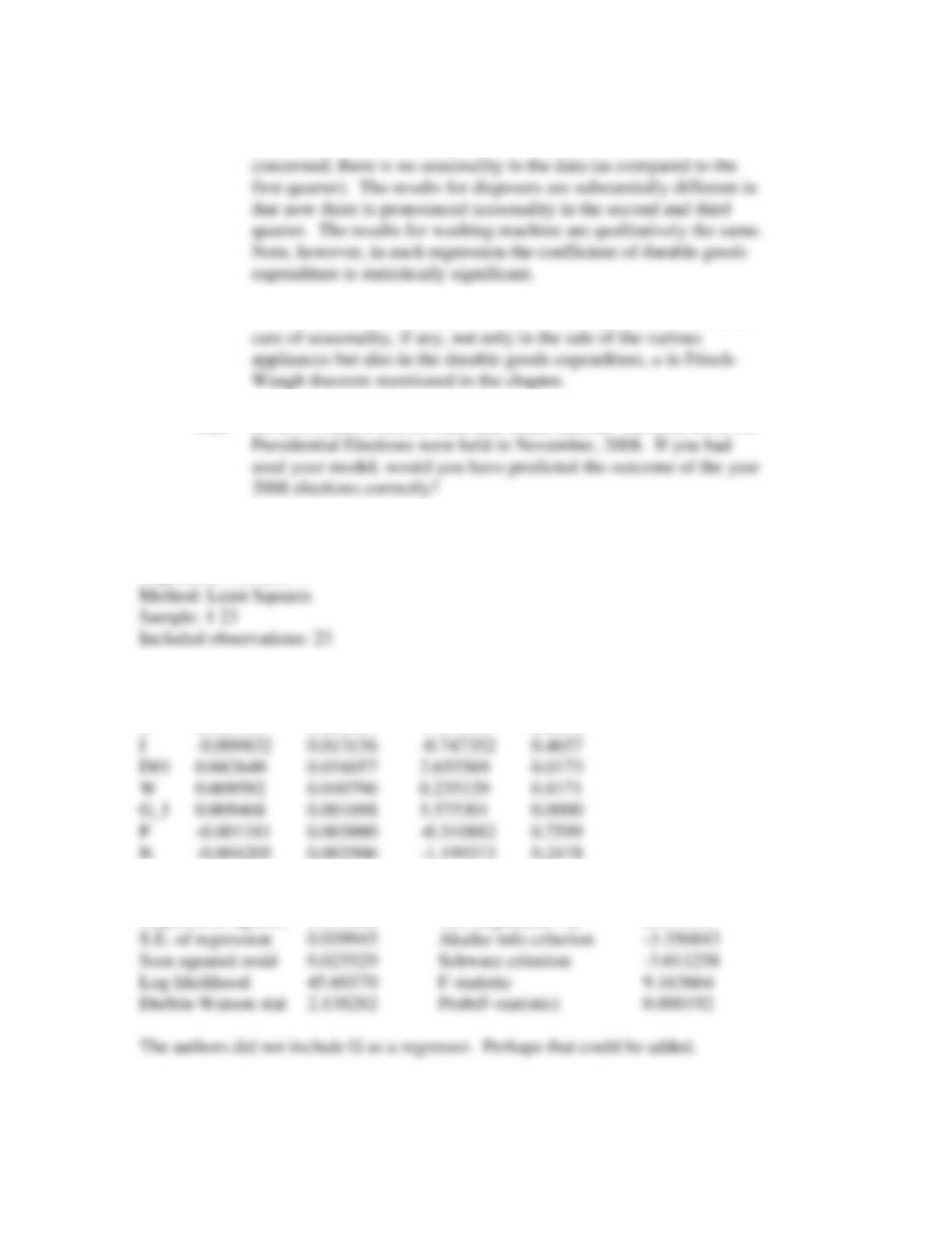
(b) The addition of expenditure on durable goods in the equation for

dishwashers does not change results insofar as seasonality is

(c) The inclusion of dummy variables in the regression model takes

9.24

(a) & (b):This is left for each individual student. The year 2008 US

(c) The results of this model are as follows:

Dependent Variable: V

Variable Coefficient Std. Error t-Statistic Prob.

C 0.509175 0.029691 17.14936 0.0000

R-squared 0.774591 Mean dependent var 0.492151

Adjusted R-squared 0.690062 S.D. dependent var 0.071750

104

9.25

The regression results based on EViews are as follows:

Dependent Variable: HWAGE

Method: Least Squares

.

Sample: 1 528

Included observations: 528

Variable Coefficient

Std. Error

t-Statistic

Prob.

C –0.261014

1.106956

-0.235794

0.8137

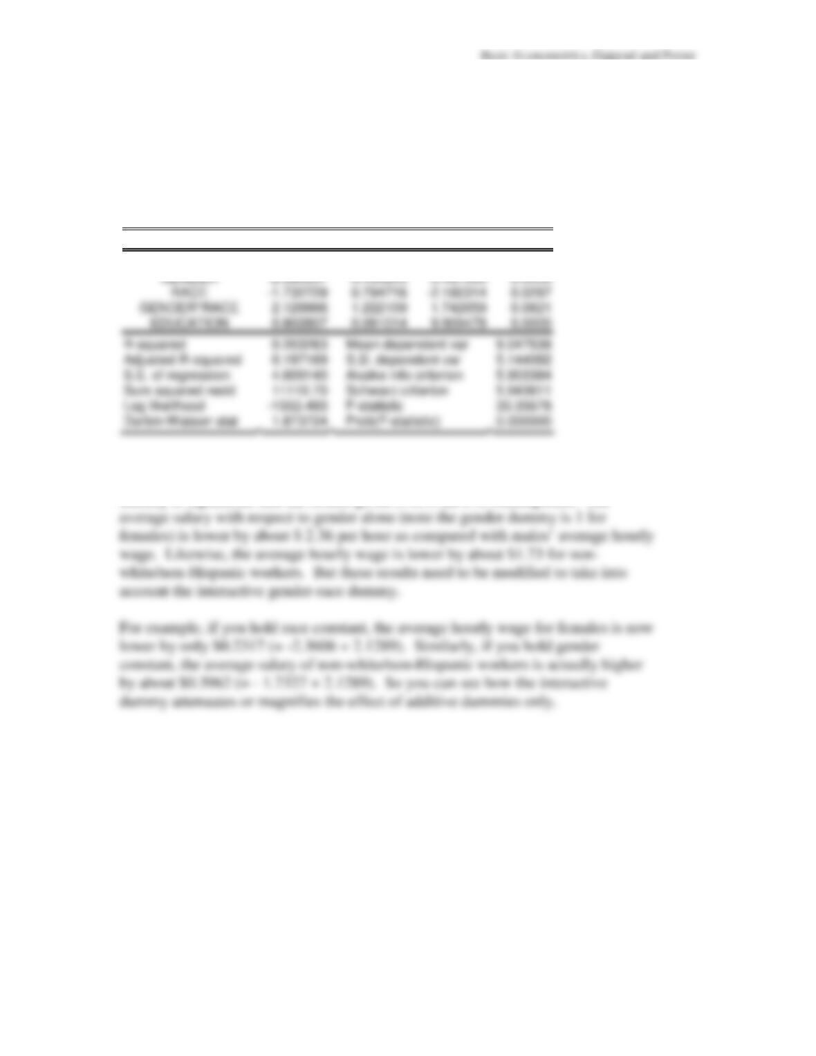
As these results show, the gender-race dummy is statistically significant at about

the 8% level. If you regard this p value as sufficiently low, then the interactive

dummy is significant and the results given (9.6.4) have to reinterpreted. The

105

9.26

The regression results, based on EViews, are as follows:

Dependent Variable: HWAGE

Method: Least Squares

.

Sample: 1 528

Included observations: 528

Variable Coefficient

Std. Error

t-Statistic

Prob.

C 9.067519

0.446115

20.32552

0.0000

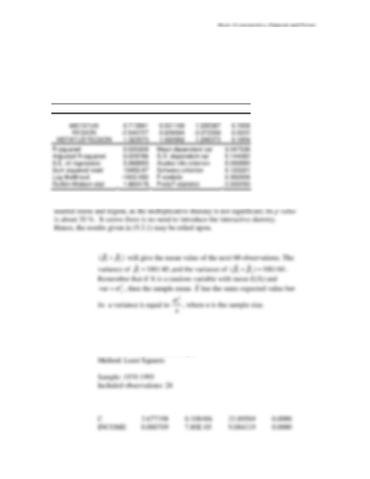
As these results suggest, there does not seem to be much interaction between

9.27

1

ˆ

β

will give the mean value of the first 40 observations and

9.28

The results, using EViews are as follows:

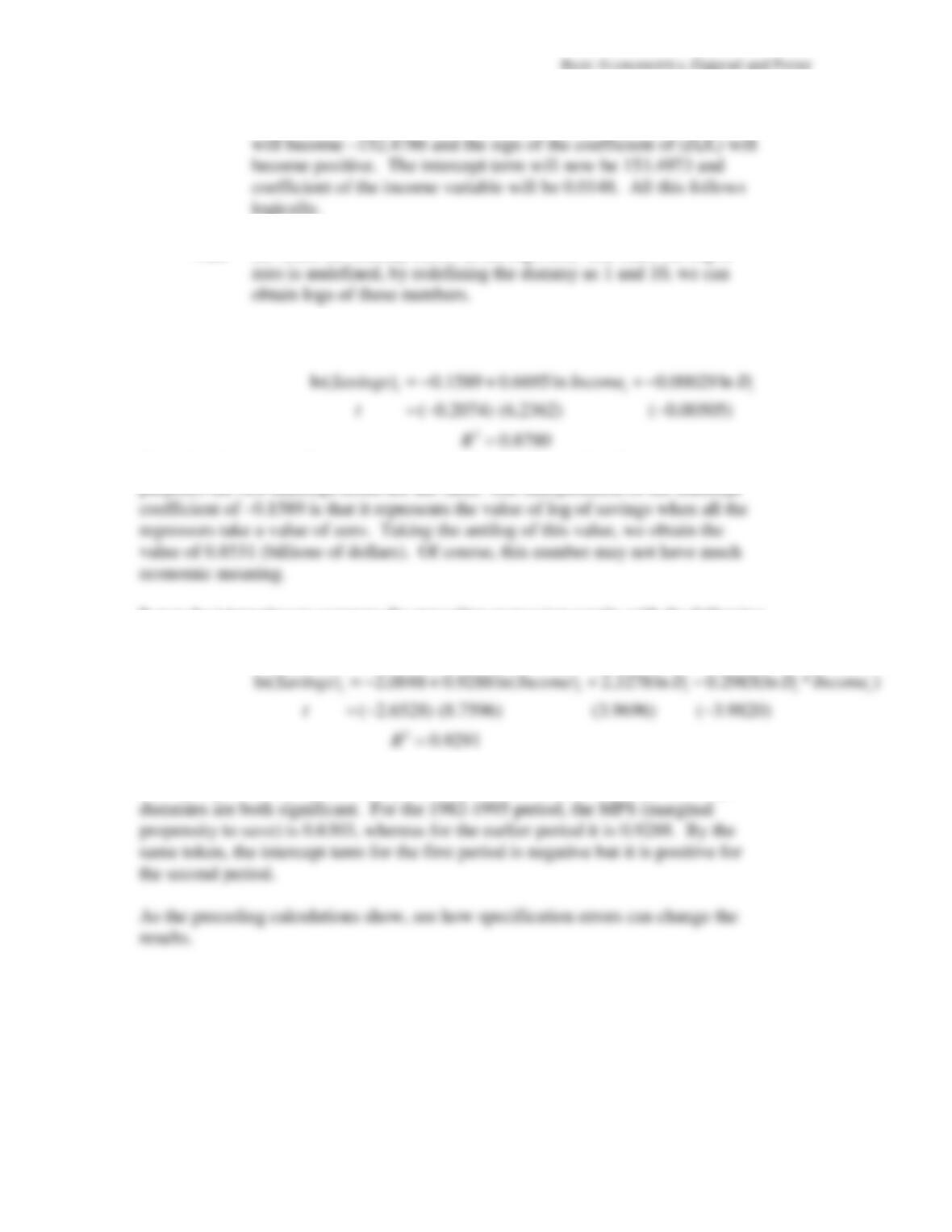
Dependent Variable: ln (Savings)

Variable Coefficient Std. Error t-Statistic Prob.

106

R-squared 0.933254 Sum squared resid 0.341255 .

F-statistic 102.5363

Durbin-Watson stat 1.612107

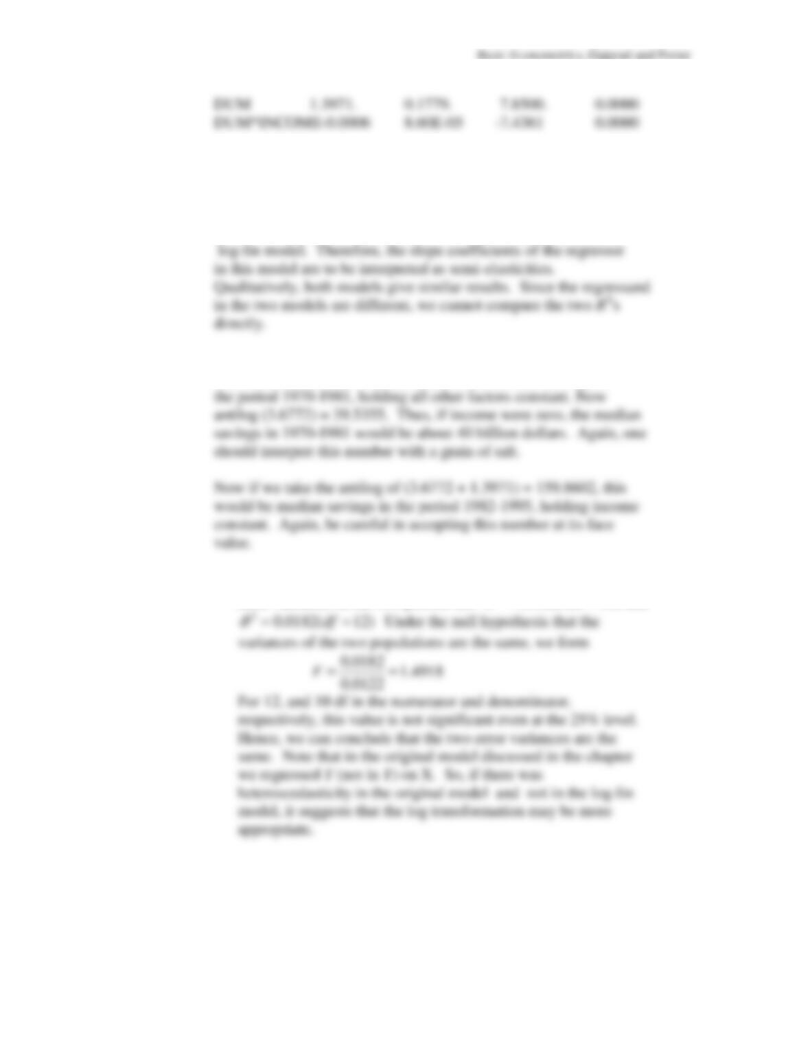
(a)

Model (9.5.4) is a linear model, whereas the present one is a

(b)

As noted in the chapter, if we take the antilog of the dummy

coefficient of 3.6772, what we obtain is the median savings in

(c)

Regressing log of Y (savings) on X (income), the estimated

error variances in the two periods are:

2

ˆ

0.0122

σ

=(df = 10) and

107

9.29

(a) Regression results using EViews are as follows:

Dependent Variable: LN_WI

Method: Least Squares

Sample: 1 114

Included observations: 114

Variable Coefficient Std. Error t-Statistic Prob.

C 3.688057 0.175749 20.98481 0.0000

AGE 0.030010 0.004734 6.339633 0.0000

R-squared 0.499976 Mean dependent var 4.648845

Adjusted R-squared 0.461879 S.D. dependent var 0.834751

Durbin-Watson stat 1.989598 Prob(F-statistic) 0.000000

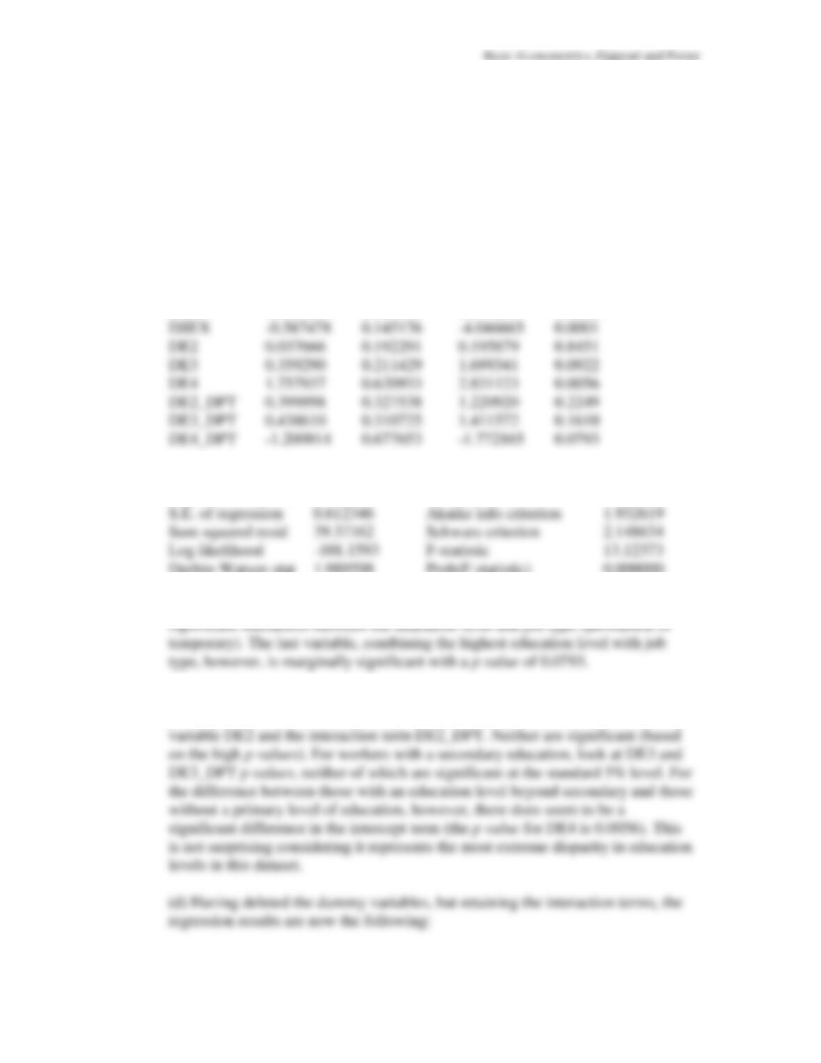
Based on the p-values of the new terms, there doesn’t really appear to be a

(b) To assess the difference between workers with an education level up to

primary and those without a primary education, we will look at both the dummy

Basic Econometrics, Gujarati and Porter

108

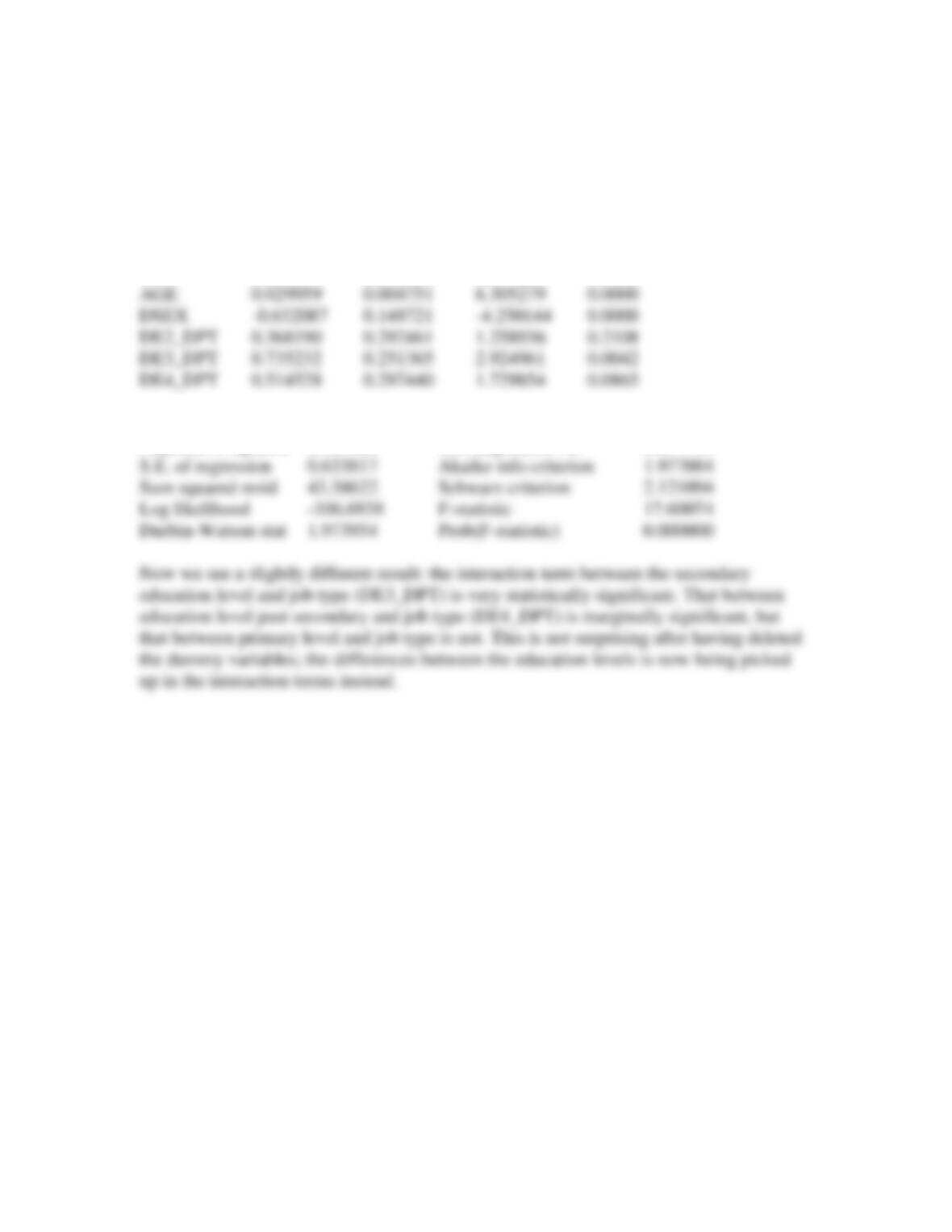
Dependent Variable: LN_WI

Method: Least Squares

Sample: 1 114

Included observations: 114

Variable Coefficient Std. Error t-Statistic Prob.

C 3.759114 0.166655 22.55621 0.0000

R-squared 0.448990 Mean dependent var 4.648845

Adjusted R-squared 0.423480 S.D. dependent var 0.834751