CHAPTER 9
A Two-Period Model: The Consumption–Savings
Decision and Credit Markets
KEY IDEAS IN THIS CHAPTER
1. Consumption smoothing yields the results that:
a) An increase in current income increases current saving as well as both current and
future consumption.
2. The Ricardian equivalence theorem states that changes in current taxes that leave the
present value of taxes constant have no effect on consumption and the real interest rate.
3. Ricardian equivalence critically depends on the idea that the burden of the public debt
is shared equally among the people alive at the time the debt is issued.
4. The burden of the debt is not shared equally when
a) There are current distributional effects of changes in taxes.
NEW IN THE FOURTH EDITION
2. New: “Macroeconomics in Action: Are Government Budget Deficits Sustainable?”
3. All charts and tables have been updated to reflect new data.
4. End-of-chapter problems have been added.
TEACHING GOALS
This chapter introduces the concept of intertemporal choice. Intertemporal choice
concerns the distribution of consumption and production of goods over more than one
time period. This chapter focuses on intertemporal consumption choice. Without a credit

Instructor’s Manual for Macroeconomics, Fourth Canadian Edition
market, each individual must consume exactly his or her current disposable income in
each and every period of time. However, many consumers would prefer to consume more
or less than their current disposable income in each period. Credit markets allow some
consumers to be better off by redistributing consumption over time. Each consumer may
also choose not to participate in the credit market, and these consumers can be no worse
off for the existence of a credit market. The existence of credit markets must therefore
allow a Pareto improvement.
An important first step for students is that they fully understand the meaning of the
intertemporal budget constraint. The first key point is that, for given amounts of income,
consumption in the present can only be changed if there is a corresponding change in
future consumption. At an intuitive level, this point is well understood by students taking
out loans for college expenses. However, students are naturally focused on making
decisions about current consumption and often lose sight of the fact that current choices
effectively preclude alternative future choices. One natural example of choice over time
is consumers’ responses to lottery winnings. Does the choice of a lump-sum payoff as
opposed to a series of annual payments affect current consumption? Does it affect current
savings? How would students respond to improved prospects for future employment
income?
Students should also understand that there is more to a change in the interest rate than an
incentive (substitution) effect acting on the returns to saving. Students should ponder the
question of who wins and who loses from changes in interest rates. Can everyone win?
Can everyone lose?
The final and often most challenging issue is Ricardian equivalence. Students often find it
difficult to conceive of tax changes that do not, at least implicitly, involve changes in
CLASSROOM DISCUSSION TOPICS
One good way to get the ball rolling is to list some macroeconomic concerns students
may have. Ask students what they think about cultural and religious admonitions against
borrowing. Should everyone respect the principle, “Neither a borrower nor a lender be?”
What about usury prohibitions on charging any interest to borrowers? There are often
tales of woe in the popular press about taking on too much consumer debt. In the modern
Chapter 9: A Two-Period Model: The Consumption–Savings Decision and Credit Markets
Ask students for their personal perspectives on the costs and benefits of government-
sponsored social security. Today’s students often believe that, while they are going to pay
a large amount of social security taxes over their lifetimes, they will receive little or
While Canadian saving is not low by OECD standards, it is much lower than that of the
fast-growing Asian economies. On average, countries with high saving rates tend to be
high-growth countries. Ask students if they can think of a reasonable explanation for this
phenomenon. Should we worry about such a low saving rate in Canada? Are there any
government policies that might promote higher a saving rate?
Several explanations for the relatively lower rate of private savings in Canada have been
Can the saving rate be raised? During World War II, the saving rate was relatively high.
This was in part due to the difficulty of buying appliances, automobiles, and other
consumer goods, since most productive capacity had been converted to war needs.

Instructor’s Manual for Macroeconomics, Fourth Canadian Edition
OUTLINE
1. The Two-Period Model
a) Consumer Behaviour
i) Consumer’s Lifetime Budget Constraint
(2) Endowment Point and the Slope of the Budget Line
ii) Consumer’s Preferences
(2) Consumers Value Diversity
(3) Current and Future Consumption are Normal Goods
iii) Consumer’s Optimization: ,’ 1
cc
M
RS r=+
iv) An Increase in Current Income
(2) Effects on Savings
(3) Excess Variability of Consumption
a. Credit Market Imperfections
b. Changes in Interest Rates
v) An Increase in Future Income
(1) Effects on Current and Future Consumption
(2) Effects on Savings
(3) Permanent Income Hypothesis
vi) An Increase in the Real Interest Rate
(1) Income Effects
(2) Substitution Effects
a. Lenders
b. Borrowers
vii) The Demand for Current Consumption Goods
b) Government Behaviour
i) Debt Issue
ii) The Government’s Present-Value Budget Constraint
c) Competitive Equilibrium
i) Consumers Optimally Choose Consumption and Savings
2. Ricardian Equivalence
a) Statement of the Theorem
b) Proof of the Theorem
Chapter 9: A Two-Period Model: The Consumption–Savings Decision and Credit Markets
i) The Distribution of Taxes across Different Individuals
TEXTBOOK QUESTION SOLUTIONS
Problems
1. Given information:
100
‘120
y
y
=
=
a) To calculate wealth, we compute:
” 110
80 180
11.1
yt
wyt r
−
=−+ = + =
+
.
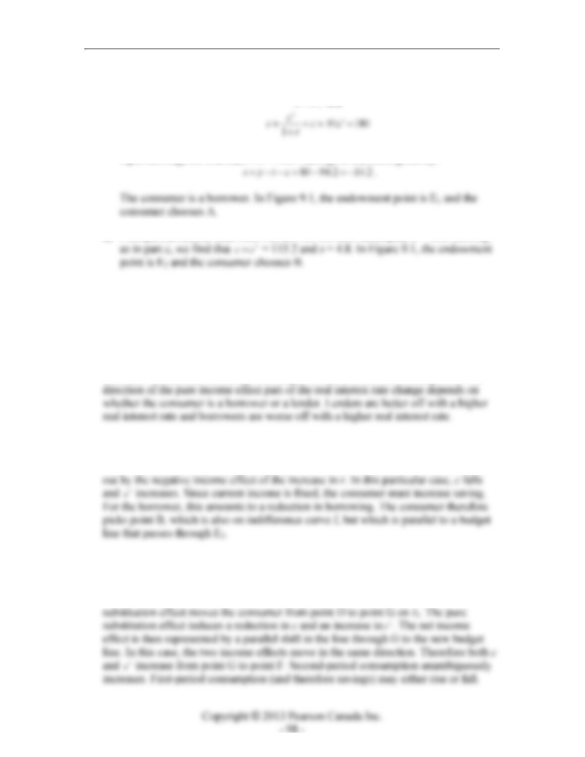
b) In the perfect complements case, the indifference curves are like I1 and I2 in
Figure 9.1.
Figure 9.1
Instructor’s Manual for Macroeconomics, Fourth Canadian Edition
c) The consumer’s optimal consumption bundle is at point A. Point A
simultaneously solves:
‘, and
cc
=
Upon solving, we find that ‘94.2cc== . Savings is therefore given by:
d) First-period income rises from 100 to 140. We now recompute w = 220. Solving
e) In part c), the consumer is a borrower. In part d), first-period income increases
and savings has consequently increased enough that the consumer is now a lender.
2. In this problem, there is a simultaneous increase in both future income and the real
interest rate. The increase in future income is a positive income effect for both
borrowers and lenders. The increase in the real interest rate includes a pure
substitution effect and a pure income effect. The substitution effect induces the
consumer to consume less in the current period and more in the second period. The
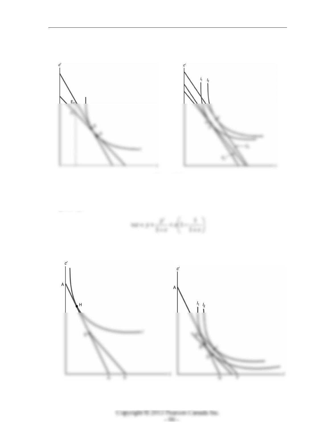
The left panel of Figure 9.2 shows the case of a borrower. The consumer starts out
with endowment E1 and picks point A on indifference curve I. The diagram
demonstrates that the positive income effect of the increase in y is exactly cancelled
The right panel of Figure 9.2 shows the case of a lender. The consumer starts out with
endowment E3. The consumer chooses point D at which the indifference curve I1 is
tangent to the budget line that passes through point E3. The disturbance shifts the
budget line out to the line that passes through E4, the new endowment point. The
Chapter 9: A Two-Period Model: The Consumption–Savings Decision and Credit Markets
The right panel of Figure 9.2 shows the case in which c increases. If c increases, s
must fall.
Figure 9.2
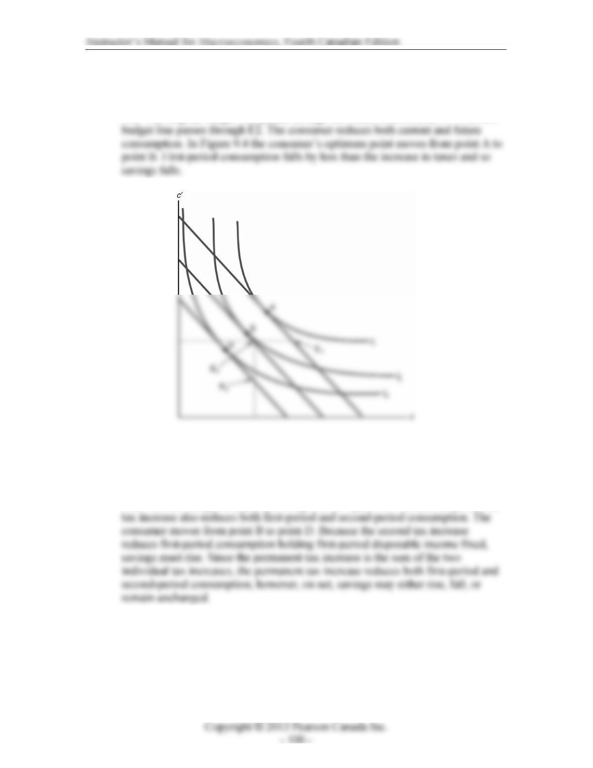
3. This problem involves a firm’s offer to provide an interest-free advance on the
consumer’s income. If the consumer takes the advance, then his lifetime wealth is
given by:
Therefore, provided that 0r>, the consumer should take the advance, as any increase
in his lifetime wealth makes him better off.
Figure 9.3
4. Temporary and Permanent Tax Increases.
a) The increase in first-period taxes induces a parallel leftward shift in the budget
line. The original budget line passes through the initial endowment, E1. The new
Figure 9.4
b) Next consider a permanent increase in taxes. A permanent tax increase adds a
second tax increase to the first tax increase, the current-period tax increase. The
increase in second-period taxes induces a parallel downward shift in the budget
line. The new budget line passes through E2 in Figure 9.4. The second part of the
5. A tax on interest income.
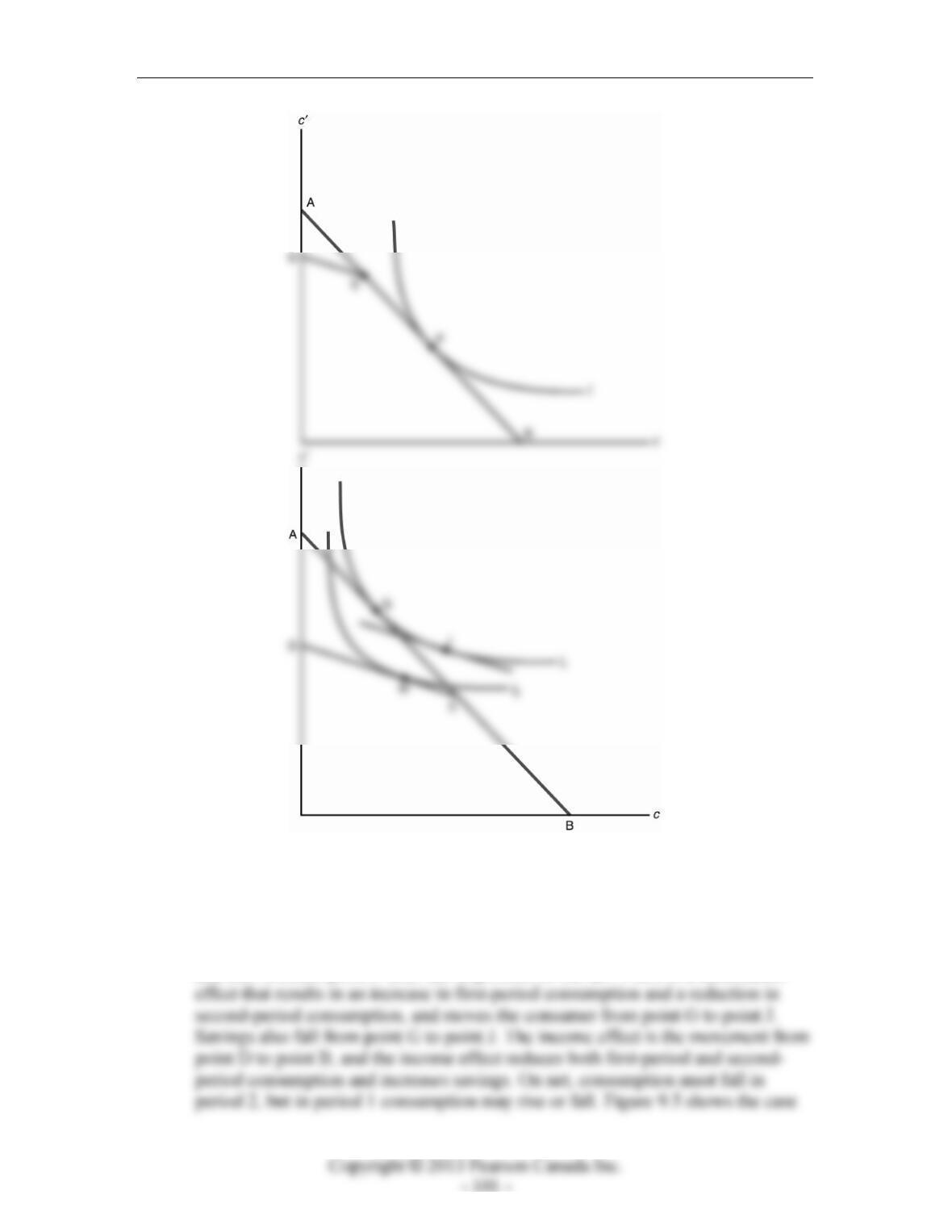
a) Initially, AB in Figure 9.5 depicts the consumer’s budget constraint. The
introduction of the tax results in a kink in the budget constraint, since the interest
rate at which the consumer can lend, (1 )rt−, is now smaller than the interest rate
at which the consumer borrows, r. The kink occurs at the endowment, E.
Chapter 9: A Two-Period Model: The Consumption–Savings Decision and Credit Markets
Figure 9.5
b) The top panel of Figure 9.5 shows the case of a consumer who was a borrower
before the imposition of the tax. This consumer is unaffected by the introduction
of the tax. The bottom panel of Figure 9.5 shows the case of a consumer who was
a lender before the imposition of the tax. Initially the consumer chooses point G,
and then chooses point H after the imposition of the tax. There is a substitution
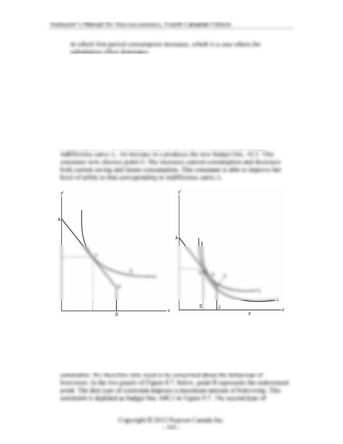
6. The consumer faces a borrowing constraint that places a ceiling on the level of
current consumption. The consumer may consume more than the current endowment,
yt−, but less than the amount of the lifetime endowment, we. The consumer’s budget
line is as in Figure 9.6, below. The budget line becomes vertical at cx=. An example
of such a budget line is depicted in the two panels of Figure 9.6 as ABD. As one
possibility, the constraint is non-binding as in the left panel of Figure 9.6. The
consumer chooses point H. A change in the level of x has no effect on such a
consumer.
Alternately, the consumer depicted in the right panel originally chooses the corner
solution, point B. The consumer achieves the level of utility corresponding to
Figure 9.6
7. This problem contrasts two alternate forms of credit market imperfections. As one
possibility, consumers may either borrow or lend at the same real interest rate, but
face a maximum amount of borrowing. The alternate possibility allows unlimited
borrowing, but the interest rate paid on borrowing exceeds the interest rate earned
from lending. Clearly, consumers who choose to be lenders are unaffected by such
Chapter 9: A Two-Period Model: The Consumption–Savings Decision and Credit Markets
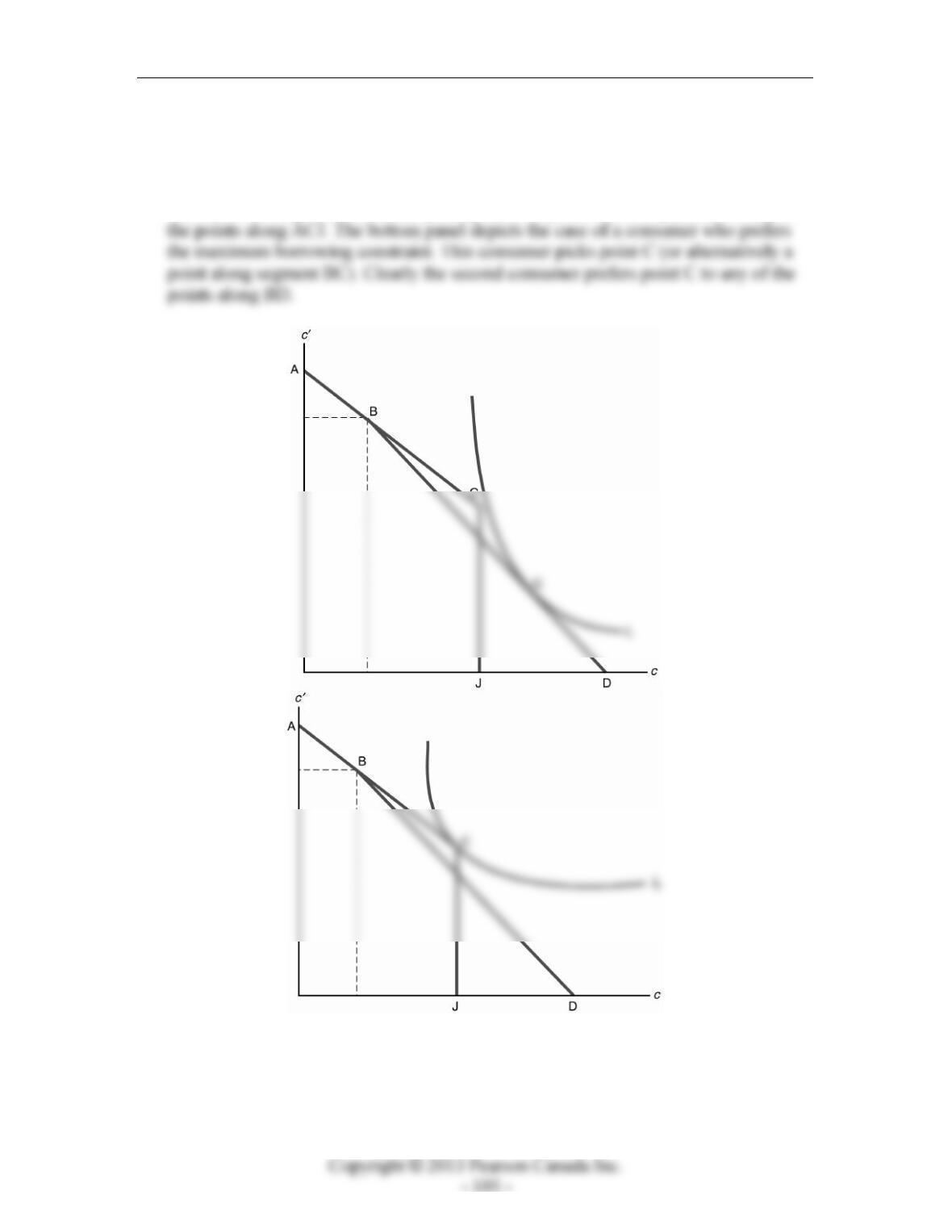
constraint imposes a higher interest rate on borrowing. This constraint is depicted as
budget line ABD in Figure 9.7.
The top panel depicts the case of a consumer who prefers to pay the higher interest
rate on borrowing. This consumer picks point G, a point which is preferred to any of
Figure 9.7

8. Given information:
200
y
=
a) If the consumer could borrow and lend at the real interest rate, r = 0.05, then the
consumer’s lifetime budget constraint would be given by:
Plugging in the numbers from this problem, we obtain:
0.95 ‘ 255.2cc+=
.
In the left panel of Figure 9.8, the initial budget constraint is given by BE1D. The
budget constraint has a kink at the initial endowment point E1 = (160,100),
Figure 9.8
b) With perfect-complements preferences, the consumer picks point A in the left
panel of Figure 9.8. Plugging c = ‘c into the budget constraint and solving, we
Chapter 9: A Two-Period Model: The Consumption–Savings Decision and Credit Markets
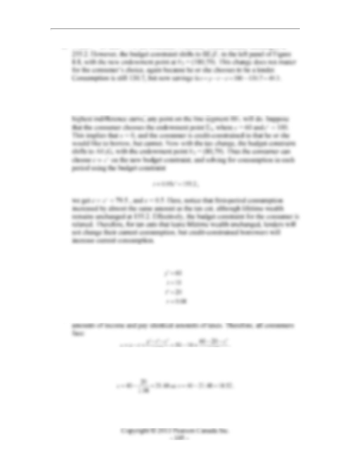
c) When t = 20 and ‘71,t= the consumer’s lifetime wealth remains unchanged at
d) Now first-period income falls to 100. Wealth is now equal to w = 155.2. In the
right panel of Figure 9.8, the budget constraint for the consumer is AE1D, so when
the consumer chooses the point on his or her budget constraint which is on the
9. Given information:
50
y
=
a) First consider the consumers’ budget constraint. All consumers receive identical
1.08 1.08
For the consumers who consume 60 in the second period:
Instructor’s Manual for Macroeconomics, Fourth Canadian Edition
For the consumers who consume 20 in the second period:
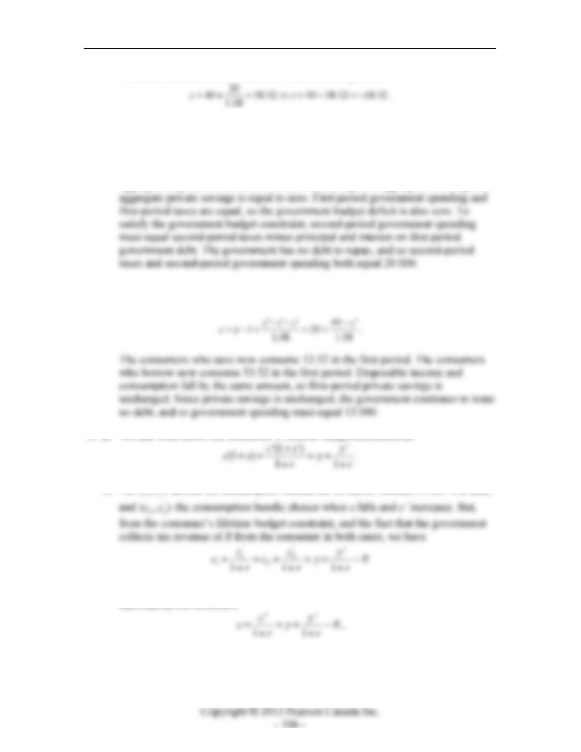
b) Aggregate first-period consumption is given by:
500 21.48 500 58.52 40, 000.C=× +× =
Total GDP for the first period is equal to 50 000. Therefore, G = 10 000. Since
aggregate disposable income (40 000) is exactly equal to aggregate consumption,
c) Assuming that consumers do not change their spending plans, we modify the
calculation from part a to obtain:
10. a) We can write down the consumer’s lifetime budget constraint as
b) Let ‘
(,)cc denote the consumption bundle the consumer chooses in the first case,
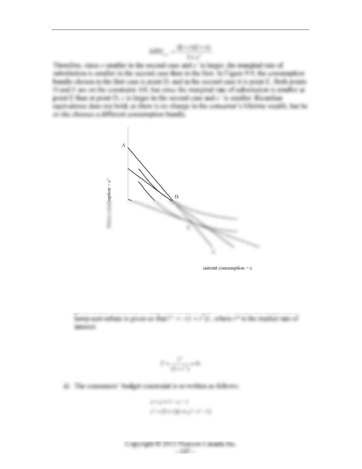
c) From part (b), the consumption allocations before and after the tax change must
but the consumer faces the budget constraint in part (a) and optimizes, so the consumer
will choose consumption in the present and the future to satisfy
Chapter 9: A Two-Period Model: The Consumption–Savings Decision and Credit Markets
11. Government loan program.
a) There is no government spending in either period. In the first period, the
government must collect lump-sum taxes so that T = L. In the second period, a
b) The present-value government budget is therefore:
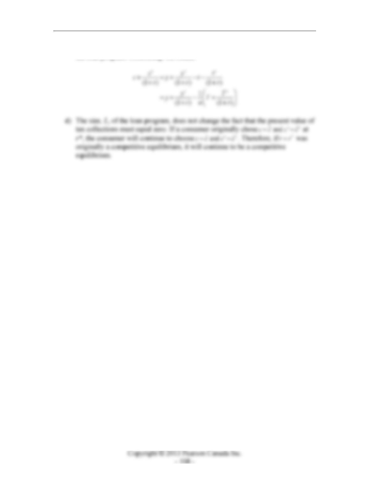
Instructor’s Manual for Macroeconomics, Fourth Canadian Edition
where
represents the size of the loan that the individual consumer takes from
the loan program. Combining, we obtain: