Questions for Review
1. When GDP declines during a recession, growth in real consumption and investment
spending both decline; unemployment rises sharply.
2. The price of a magazine is an example of a price that is sticky in the short run and flex-
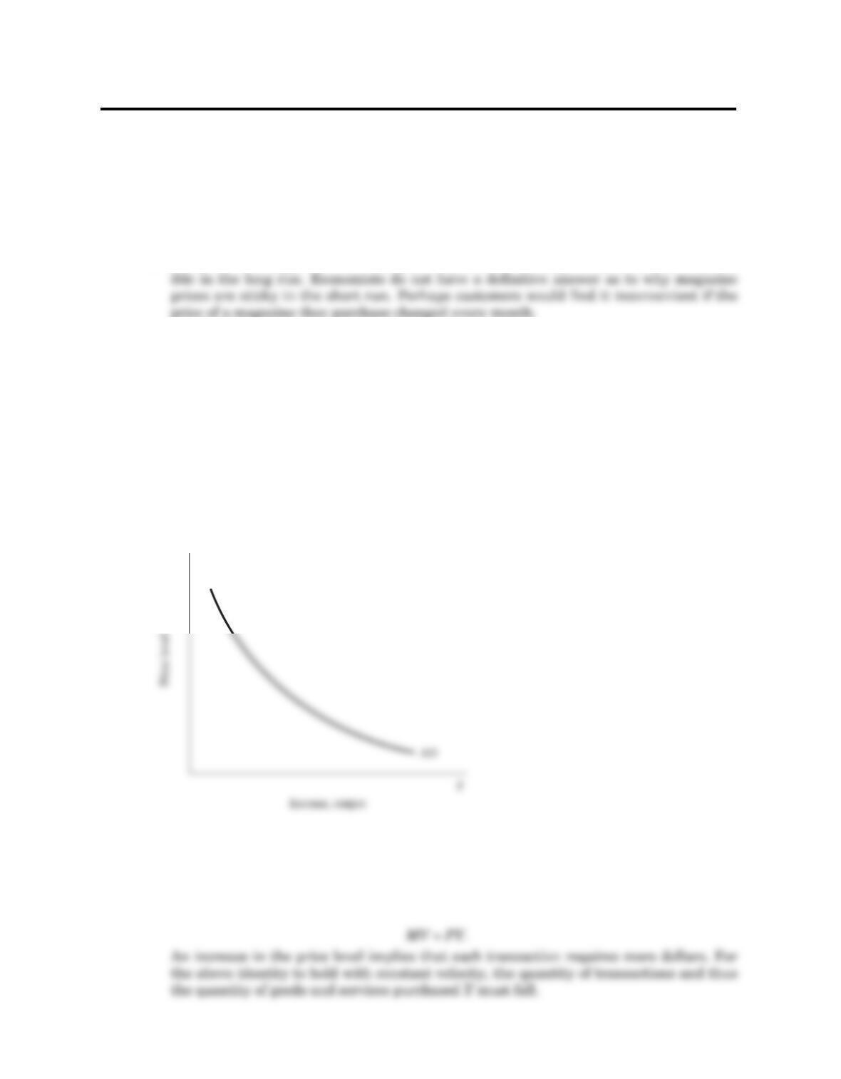
3. Aggregate demand is the relation between the quantity of output demanded and the
aggregate price level. To understand why the aggregate demand curve slopes down-
ward, we need to develop a theory of aggregate demand. One simple theory of aggre-
gate demand is based on the quantity theory of money. Write the quantity equation in
terms of the supply and demand for real money balances as
M/P = (M/P)d= kY,
where k= 1/V. This equation tells us that for any fixed money supply M, a negative
relationship exists between the price level Pand output Y, assuming that velocity Vis
fixed: the higher the price level, the lower the level of real balances and, therefore, the
lower the quantity of goods and services demanded Y. In other words, the aggregate
demand curve slopes downward, as in Figure 9–1.
One way to understand this negative relationship between the price level and out-
put is to note the link between money and transactions. If we assume that Vis con-
stant, then the money supply determines the dollar value of all transactions:
77
P
Figure 9–1
CHAPTER 9Introduction to Economic Fluctuations
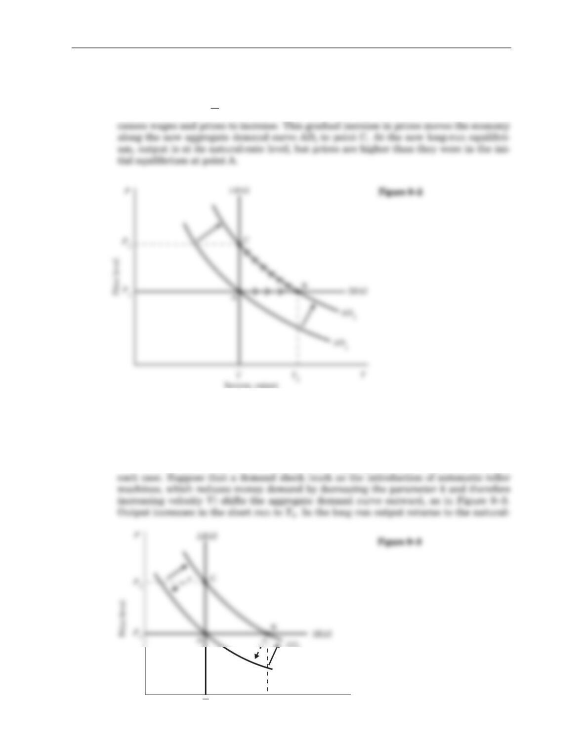
4. If the Fed increases the money supply, then the aggregate demand curve shifts out-
ward, as in Figure 9–2. In the short run, prices are sticky, so the economy moves along
the short-run aggregate supply curve from point A to point B. Output rises above its
natural rate level Y: the economy is in a boom. The high demand, however, eventually
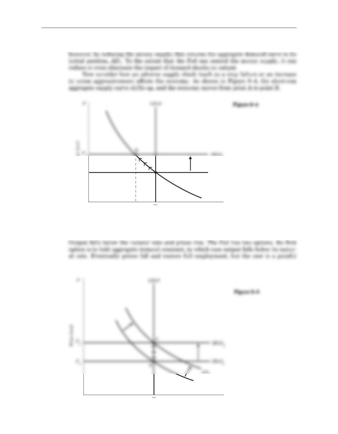
5. It is easier for the Fed to deal with demand shocks than with supply shocks because the
Fed can reduce or even eliminate the impact of demand shocks on output by controlling
the money supply. In the case of a supply shock, however, there is no way for the Fed to
adjust aggregate demand to maintain both full employment and a stable price level.
To understand why this is true, consider the policy options available to the Fed in
78 Answers to Textbook Questions and Problems
Y
Income, output
Y2
Y
AD1
rate level, but at a higher price level P2. The Fed can offset this increase in velocity,
Chapter 9 Introduction to Economic Fluctuations 79
Price level
A
AD
Y
Income, output
P1
SRAS1
Y
Y2
YY
Income, output
AD1
recession. Its second option is to increase aggregate demand by increasing the money
supply, bringing the economy back toward the natural rate of output, as in Figure 9–5.
This policy leads to a permanently higher price level at the new equilibrium, point
C. Thus, in the case of a supply shock, there is no way to adjust aggregate demand to
maintain both full employment and a stable price level.
Problems and Applications
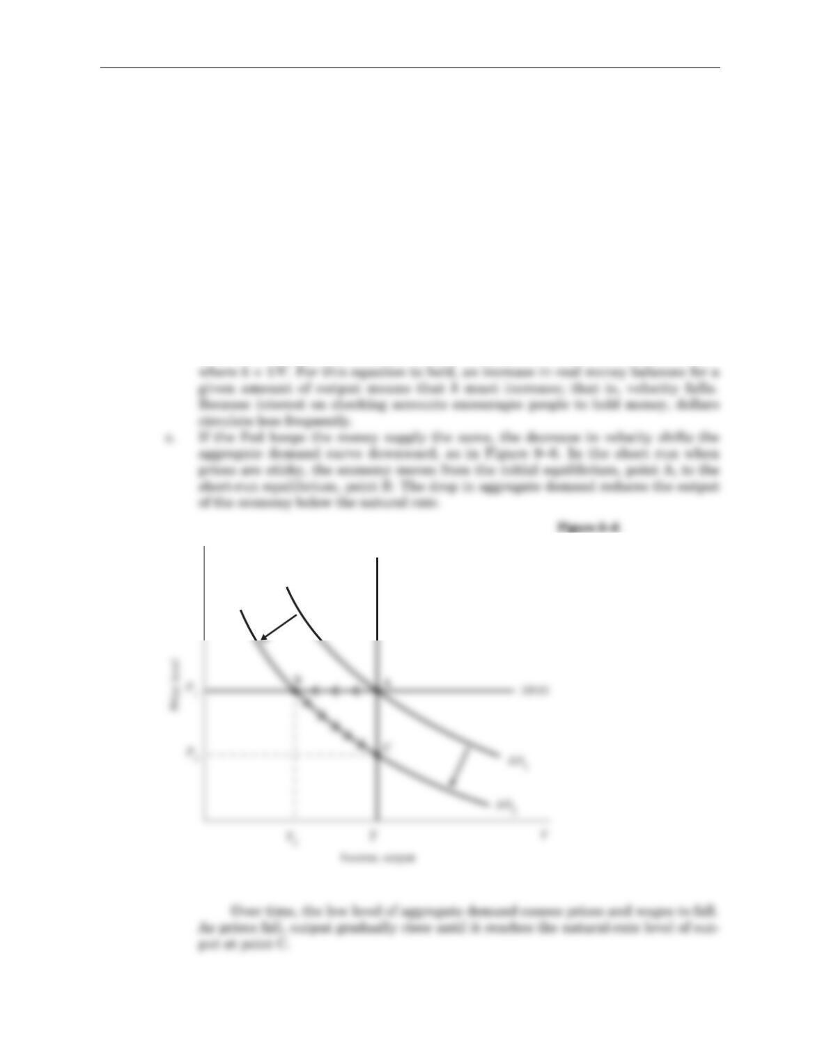
1. a. Interest-bearing checking accounts make holding money more attractive. This
increases the demand for money.
b. The increase in money demand is equivalent to a decrease in the velocity of
money. Recall the quantity equation
M/P = kY,
80 Answers to Textbook Questions and Problems
LRASP
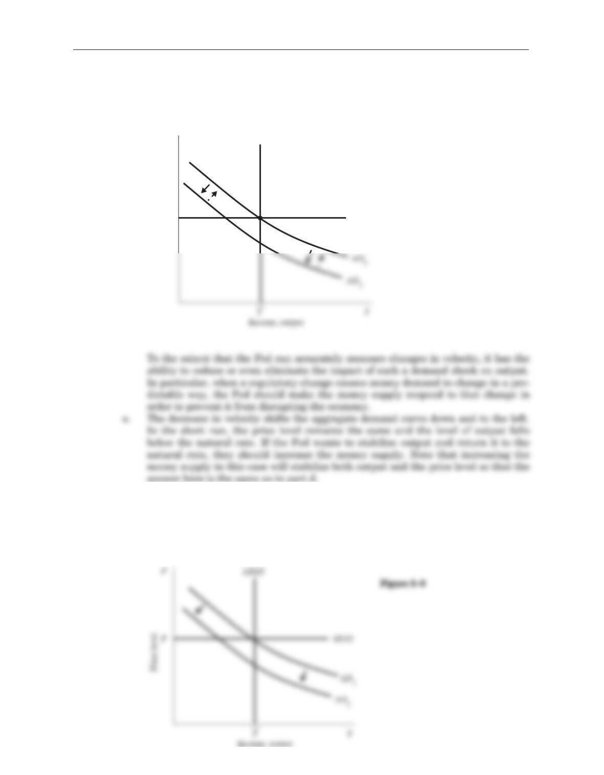
d. The decrease in velocity causes the aggregate demand curve to shift downward.
The Fed could increase the money supply to offset this decrease and thereby
return the economy to its original equilibrium at point A, as in Figure 9–7.
2. a. If the Fed reduces the money supply, then the aggregate demand curve shifts
down, as in Figure 9–8. This result is based on the quantity equation MV = PY,
which tells us that a decrease in money Mleads to a proportionate decrease in
nominal output PY (assuming that velocity Vis fixed). For any given price level P,
the level of output Yis lower, and for any given Y, Pis lower.
Chapter 9 Introduction to Economic Fluctuations 81
SRAS
A
LRAS
P
Price level
Figure 9–7
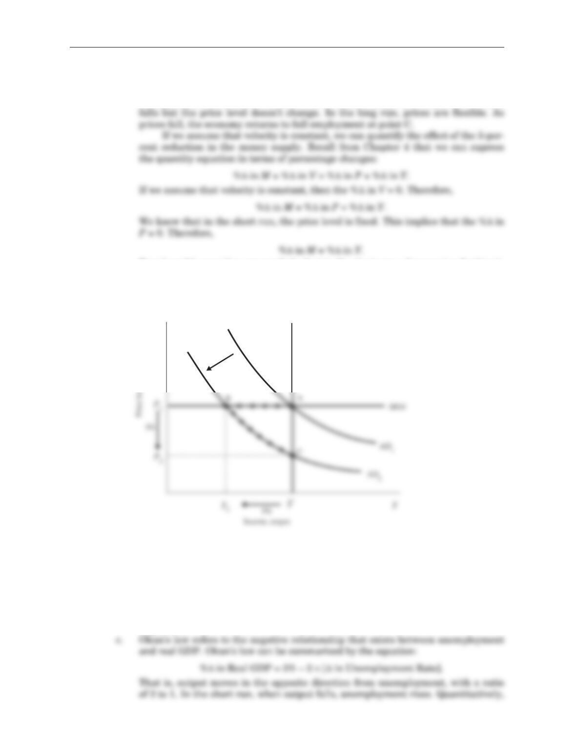
b. In the short run, we assume that the price level is fixed and that the aggregate
supply curve is flat. As Figure 9–9 shows, in the short run, the leftward shift in
the aggregate demand curve leads to a movement from point A to point B—output
Based on this equation, we conclude that in the short run a 5-percent reduction in
the money supply leads to a 5-percent reduction in output. This is shown in
Figure 9–9.
In the long run we know that prices are flexible and the economy returns to
its natural rate of output. This implies that in the long run, the %Δin Y= 0.
Therefore,
%Δin M= %Δin P.
Based on this equation, we conclude that in the long run a 5-percent reduction in
the money supply leads to a 5-percent reduction in the price level, as shown in
Figure 9–9.
82 Answers to Textbook Questions and Problems
P
LRAS
P
Figure 9–9
if velocity is constant, we found that output falls 5 percentage points relative to
full employment in the short run. Okun’s law states that output growth equals the
full employment growth rate of 3 percent minus two times the change in the
unemployment rate. Therefore, if output falls 5 percentage points relative to full-
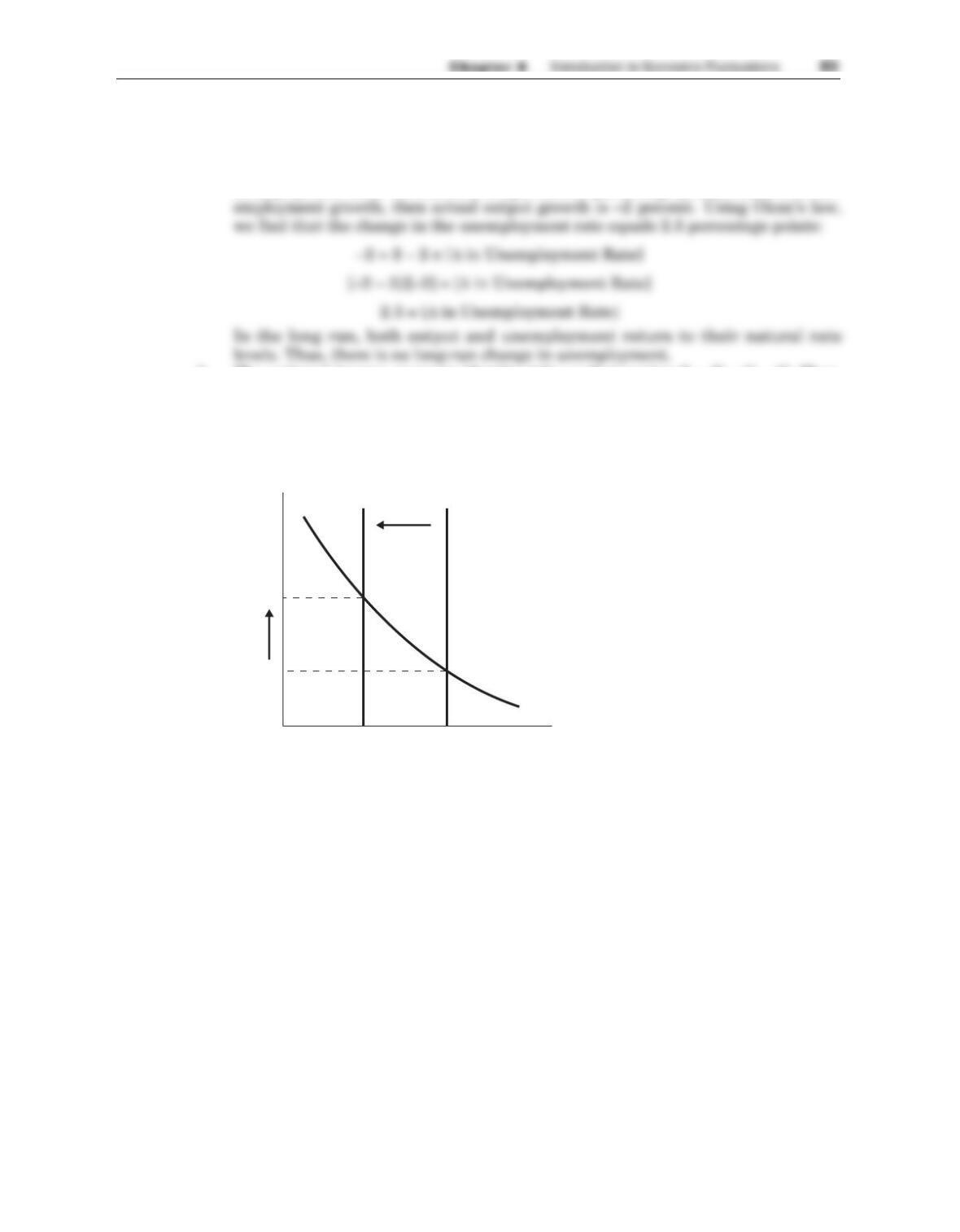
d. The national income accounts identity tells us that saving S= Y– C– G. Thus,
when Yfalls, Sfalls (assuming the marginal propensity to consume is less than
one). Figure 9–10 shows that this causes the real interest rate to rise. When Y
returns to its original equilibrium level, so does the real interest rate.
I, S
Investment, Saving
Real interest rate
r
I(r)
r1
r2
S2S1
Figure 9–10
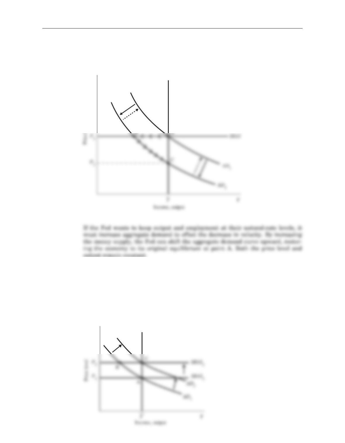
3. a. An exogenous decrease in the velocity of money causes the aggregate demand
curve to shift downward, as in Figure 9–11. In the short run, prices are fixed, so
output falls.
If the Fed wants to keep prices stable, then it wants to avoid the long-run
adjustment to a lower price level at point C in Figure 9–11. Therefore, it should
increase the money supply and shift the aggregate demand curve upward, again
restoring the original equilibrium at point A.
Thus, both Feds make the same choice of policy in response to this demand
shock.
b. An exogenous increase in the price of oil is an adverse supply shock that causes
the short-run aggregate supply curve to shift upward, as in Figure 9–12.
PLRAS
Figure 9–12
84 Answers to Textbook Questions and Problems
LRAS
P
Figure 9–11
If the Fed cares about keeping output and employment at their natural-rate
levels, then it should increase aggregate demand by increasing the money supply.
This policy response shifts the aggregate demand curve upwards, as shown in the
P1. But the cost of this process is a prolonged recession.
Thus, the two Feds make a different policy choice in response to a supply
shock.
4. From the main NBER web page (www.nber.org), I followed the link to Business
Cycle Dates (downloaded February 19, 2009). As of this writing, the latest turning
Chapter 9 Introduction to Economic Fluctuations 85