Economics Chapter 9 Homework By multiplying it out, we find that the matrix of

Chapter 9

The Generalized Regression Model

and Heteroscedasticity

◼ Exercises

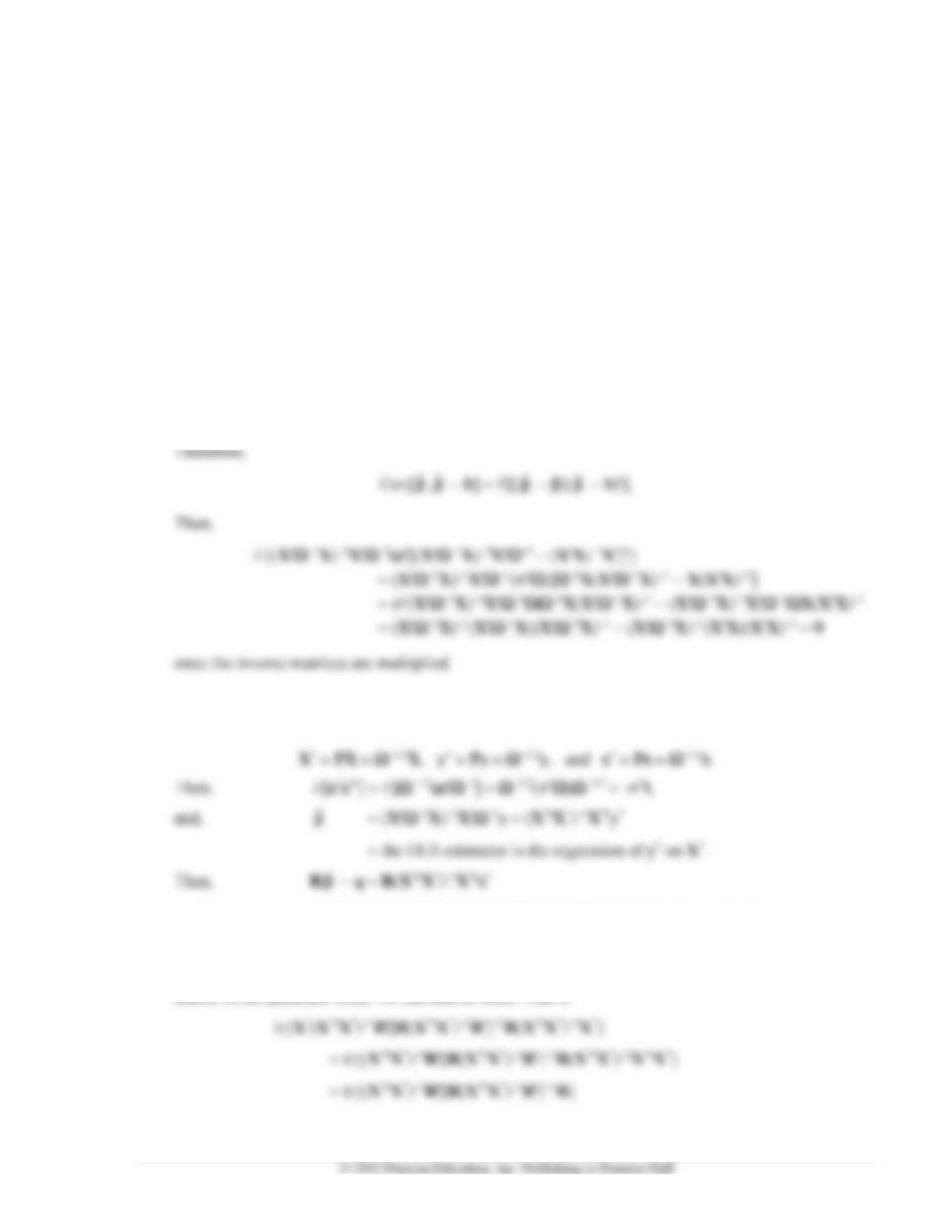
1. Write the two estimators as

ˆ



=  + (X−1X)−1X−1 and b =  + (XX)−1X. Then,

(

ˆ



− b) = [(X−1X)−1X−1 − (XX)− 1X]  has E [

ˆ



− b] = 0 since both estimators are unbiased.

2. First, (R

ˆ



− q) = R[ + (X−1X)−1X−1] − q = R(X−1X)−1X−1 if R − q = 0.

Now, use the inverse square root matrix of , P = −1/2 to obtain the transformed data,

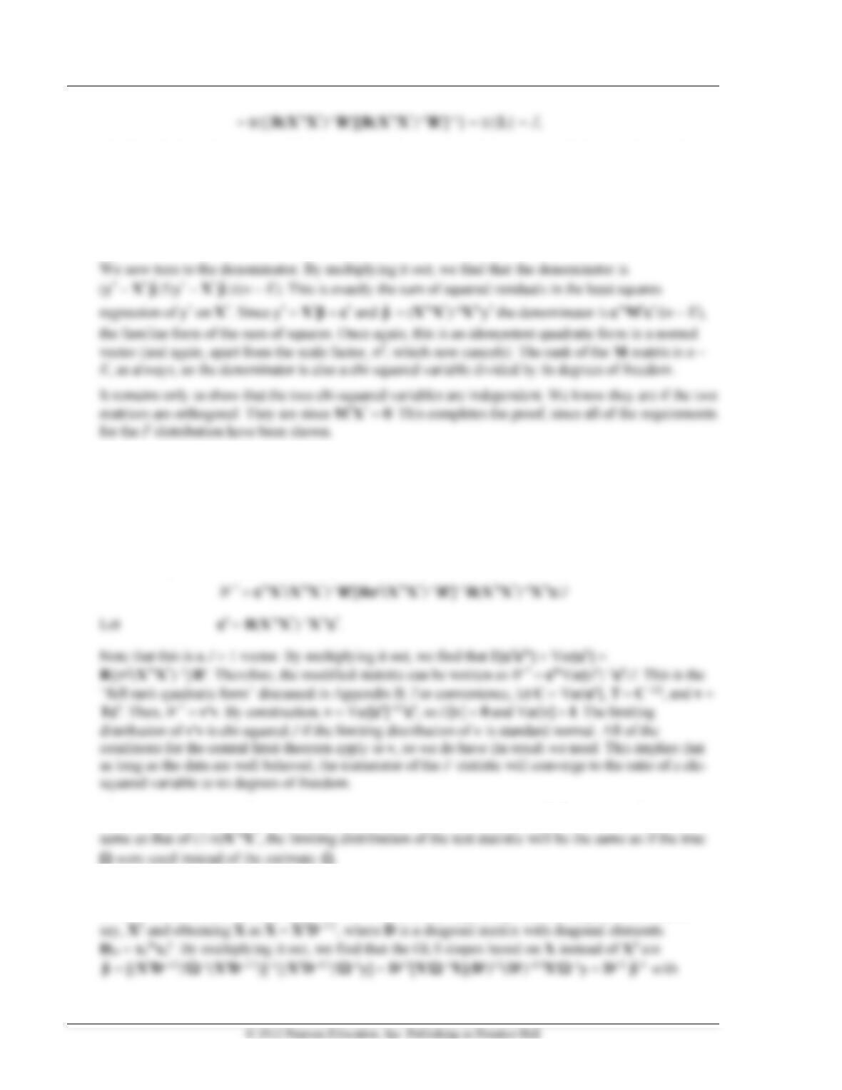
and the numerator is *X*(X*X*)−1R[R(X*X*)−1R]−1R(X*X*)−1X**/J. By multiplying it out, we

find that the matrix of the quadratic form above is idempotent. Therefore, this is an idempotent

quadratic form in a normally distributed random vector. Thus, its distribution is that of 2 times a chi-

squared variable with degrees of freedom equal to the rank of the matrix. To find the rank of the

matrix of the quadratic form, we can find its trace. That is

64 Greene • Econometric Analysis, Seventh Edition

which might have been expected. Before proceeding, we should note, we could have deduced this

outcome from the form of the matrix. The matrix of the quadratic form is of the form Q = X*ABAX*

where B is the nonsingular matrix in the square brackets and A = (X*X*)−1R, which is a K  J matrix

which cannot have a rank higher than J. Therefore, the entire product cannot have a rank higher than J.

Continuing, we now find that the numerator (apart from the scale factor, 2) is the ratio of a

chi-squared [J] variable to its degrees of freedom.

3. First, we know that the denominator of the F statistic converges to 2. Therefore, the limiting distribution

of the F statistic is the same as the limiting distribution of the statistic which results when the denominator

is replaced by 2. It is useful to write this modified statistic as

W * = (1/2)(R

ˆ



− q)[R(X*X*)−1R]−1(R

ˆ



− q)/J.

Now, incorporate the results from the previous problem to write this as

4. The development is unchanged. As long as the limiting behavior of (1/n)

ˆˆ



XX

= (1/n)X

ˆ



−1X is the

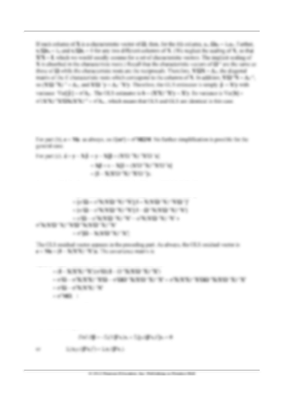
5. First, in order to simplify the algebra somewhat without losing any generality, we will scale the

columns of X so that for each xk, xkxk = 1. We do this by beginning with our original data matrix,

Chapter 9 The Generalized Regression Model and Heteroscedasticity 65

66 Greene • Econometric Analysis, Seventh Edition

6. Write b =  + (XX)−1X and

ˆ



=  + (X−1X)−1X −1. The covariance matrix is

E[(b − )(

ˆ



− )] = E[(XX)−1X −1X(X−1X)−1] = (XX)−1X(2)−1X(X−1X)−1 =

2(X−1X)−1.

Thus, E[

ˆ



ˆ



] = [I − X(X−1X)−1X−1]E[][I − X(X−1X)−1X−1]

= [I − X(X−1X)−1X−1](2)[I − X(X−1X)−1X−1]

E[e

ˆ



] = E[(I − X(XX)−1X)(I − X(X−1X)−1X−1)]

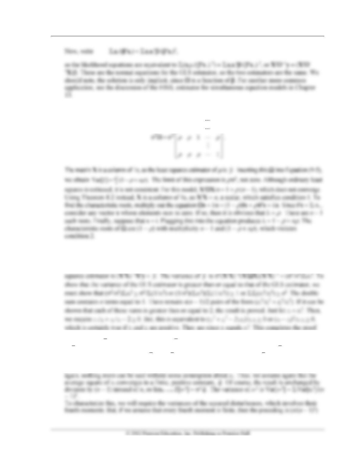
7. The GLS estimator is

ˆ



= (X−1X)−1X−1y = [ixixi/(xi)2]−1[ixiyi/(xi)2]. The log likelihood for

this model is lnL = −iln(xi) − iyi/(xi).

The likelihood equations are

Chapter 9 The Generalized Regression Model and Heteroscedasticity 67

8. The covariance matrix is

1

  





9. This is a heteroscedastic regression model in which the matrix X is a column of ones. The efficient

estimator is the GLS estimator,

ˆ



= (X−1X)−1X−1y = [i1yi/xi2]/[i 12/xi2] = [i(yi/xi2)]/[i(1/xi2)].

As always, the variance of the estimator is Var[

ˆ



] = 2(X−1X)−1 = 2/[i(1/xi2)]. The ordinary least

10. Consider first,

.y

We saw earlier that Var[

y

] = (2/n2)ixi2 = (2/n)(1/n)ixi2. The expected value is

E[

y

] = E[(1/n)iyi] = . If the mean square of x converges to something finite, then

y

is consistent

for . That is, if plim(1/n)ixi2 =

q

where

q

is some finite number, then, plim

y

.q

= . As such, it

follows that s2 and s*2 = (1/(n − 1))i(yi − )2 have the same probability limit. We consider, therefore,

plim s*2 = plim(1/(n − 1))ii2. The expected value of s*2 is E[(1/(n − 1)) ii2] = 2(1/ixi2). Once

68 Greene • Econometric Analysis, Seventh Edition

11. The residuals from the least squares regression are ei = yi −

y

=  + i − ( +



) = i −



The expected value of the squared residual is

E[ei2] = E[i2] + E[

2



] − 2E[i



] = i2 + (1/n2)E[(ii)2] − (2/n)E[i(jj)]

= i2 + (1/n2)I E[i2] − (2/n)E[i2]

since the disturbances are uncorrelated. We can write this as

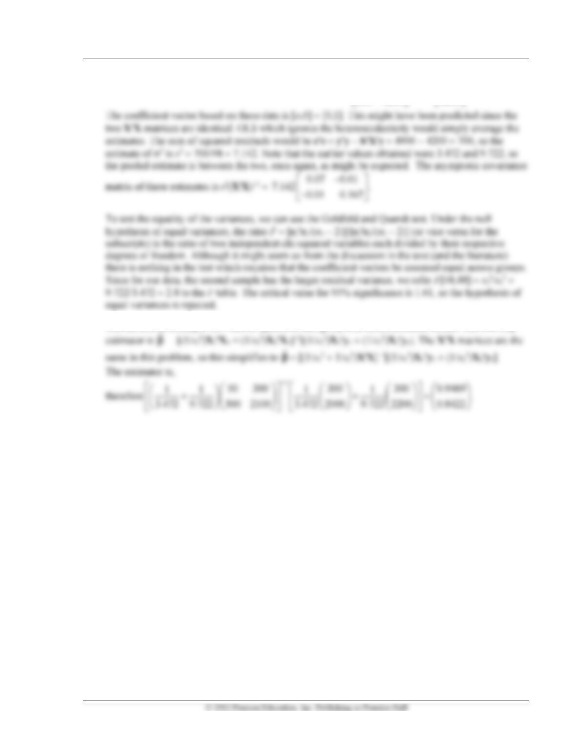
12. The sample moments are obtained using, for example, Sxx = xx − n

2,x

and so on. For the two samples,

we obtain

y

x

Sxx Syy Sxy

The parameter estimates are computed directly using the results of Chapter 6.

Intercept Slope R2 s2

Chapter 9 The Generalized Regression Model and Heteroscedasticity 69

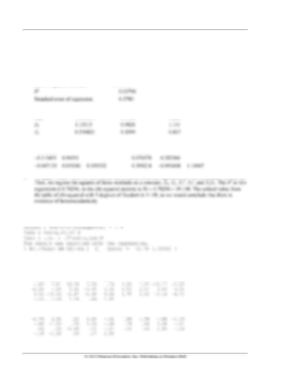
The pooled moments based on 100 observations are

   



= = =

   

100 600 600

, , 4900.

600 4200 4200

X X Xy y y

The method of Example 12.9 can be applied to this groupwise heteroscedastic model. The two step

70 Greene • Econometric Analysis, Seventh Edition

Applications

?=======================================================

? Application 9.1

?=======================================================

a. The ordinary least squares regression of Y on a constant, X1, and X2 produces the following results:

Sum of squared residuals 1911.9275

Variable Coefficient Standard Error t-ratio

One 0.190394 0.9144 0.208

b. Covariance Matrix White’s Corrected Matrix

0.836212 0.524589

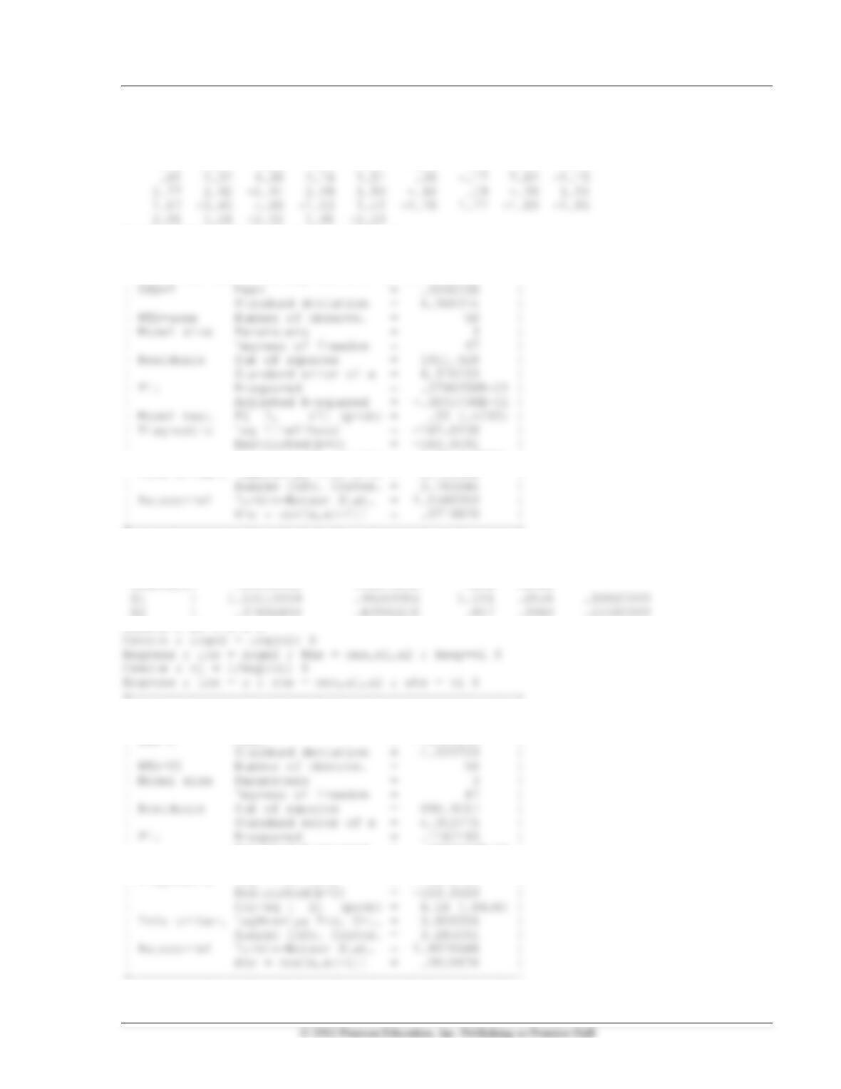
c. To apply White’s test, we first obtain the residuals from the regression of Y on a constant, X1, and X2.

d. Lagrange multiplier test

Regress;Lhs=y;rhs=one,x1,x2 ; Res=e ; het $

e. Two-step estimator

read;nobs=50;nvar=1;names=y;byva $

-1.42 2.75 2.10 –5.08 1.49 1.00 .16 -1.11 1.66

-.26 -4.87 5.94 2.21 -6.87 .90 1.61 2.11 –3.82

read;nobs=50;nvar=1;names=x1;byva $

-1.65 1.48 .77 .67 .68 .23 –.40 –1.13 .15

-.63 .34 .35 .79 .77 -1.04 .28 .58 –.41

Chapter 9 The Generalized Regression Model and Heteroscedasticity 71

read;nobs=50;nvar=1;names=x2;byva $

-.67 .70 .32 2.88 -.19 –1.28 –2.72 –.70 –1.55

-.74 -1.87 1.56 .37 -2.07 1.20 .26 -1.34 –2.10

Regress;Lhs=y;rhs=one,x1,x2 ; Res=e $

+—————————————————-+

| Ordinary least squares regression |

| Model was estimated May 12, 2007 at 08:33:20PM |

| Chi-sq [ 2] (prob) = 1.93 (.3806) |

| Info criter. LogAmemiya Prd. Crt. = 3.763988 |

+—————————————————-+

+——–+————–+—————-+——–+——–+———-+

+——–+————–+—————-+——–+——–+———-+

Create ; e2 = e*e $

+—————————————————-+

| Ordinary least squares regression |

| Model was estimated May 12, 2007 at 08:33:20PM |

| LHS=Y Mean = -.5316339 |

| Adjusted R-squared = .7861157E-01 |

| Model test F[ 2, 47] (prob) = 3.09 (.0548) |

| Diagnostic Log likelihood = -150.0732 |

+—————————————————-+

72 Greene • Econometric Analysis, Seventh Edition

+——–+————–+—————-+——–+——–+———-+

+——–+————–+—————-+——–+——–+———-+

Constant| .16662621 .71981411 .231 .8179

?=======================================================

Application 9.2

?=======================================================

The procedure is shown in Section 14.9.2.a.

create ; lc=log(c);lq=log(q);lq2=lq*lq;lpf=log(pf)$

Proc

create ; wti=1/exp(d’z) $

regr ; quietly ; lhs = lc ; rhs = one,lq,lq2,lpf ; wts = wti ; res = e$

create ; e2=e^2/exp(d’z)- 1 $

[CALC] CHANGE = 4.0934839

[CALC] CHANGE = 8.9498852

[CALC] CHANGE = 9.5669462

Chapter 9 The Generalized Regression Model and Heteroscedasticity 73

-> regr ; lhs = lc ; rhs = one,lq,lq2,lpf ; wts = wti ; res = e$

—————————————————————————–

Ordinary least squares regression …………

LHS=LC Mean = 12.99902

Standard deviation = 1.19008

——–+——————————————————————–

| Standard Prob. 95% Confidence

LC| Coefficient Error t |t|>T* Interval

——–+——————————————————————–

Constant| 9.26108*** .21476 43.12 .0000 8.84016 9.68200

—————————————————————————–

User Specified Model

——–+——————————————————————–

| Standard Prob. 95% Confidence

LC| Coefficient Error z |z|>Z* Interval

——–+——————————————————————–

Constant| -9.59229*** 1.59839 -6.00 .0000 -12.72508 -6.45951

—————————————————————————–