CHAPTER 8
TEACHING NOTES
This is a good place to remind students that homoskedasticity played no role in showing that
OLS is unbiased for the parameters in the regression equation. In addition, you probably should
discuss how there is nothing wrong with the R-squared or adjusted R-squared as goodness-of-fit
By explicitly stating the homoskedasticity assumption as conditional on the explanatory
variables that appear in the conditional mean, it is clear that only heteroskedasticity that depends
As I mention in the text, other traditional tests for heteroskedasticity, such as the Park and
Glejser tests, do not directly test what we want, or add too many assumptions under the null. The
Goldfeld-Quandt test only works when there is a natural way to order the data based on one
independent variable. This is rare in practice, especially for cross-sectional applications.
Some argue that weighted least squares estimation is a relic, and is no longer necessary given the
Weighted least squares estimation of the LPM is a nice example of feasible GLS, at least when
all fitted values are in the unit interval. Interestingly, in the LPM examples in the text and the
90
SOLUTIONS TO PROBLEMS
8.1 Parts (ii) and (iii). The homoskedasticity assumption played no role in Chapter 5 in showing
8.2 With Var(u|inc,price,educ,female) =
2inc2, h(x) = inc2, where h(x) is the heteroskedasticity
8.3 False. The unbiasedness of WLS and OLS hinges crucially on Assumption MLR.4, and, as
we know from Chapter 4, this assumption is often violated when an important variable is
8.4 (i) These coefficients have the anticipated signs. If a student takes courses where grades are,
on average, higher – as reflected by higher crsgpa – then his/her grades will be higher. The
(ii) This is easiest to see without other explanatory variables in the model. If crsgpa were the
(iii) The in-season effect is given by the coefficient on season, which implies that, other
8.5 (i) No. For each coefficient, the usual standard errors and the heteroskedasticity-robust ones
are practically very similar.
(v) We just plug the values of the independent variables into the OLS regression line:
8.6 (i) The proposed test is a hybrid of the BP and White tests. There are k + 1 regressors, each
original explanatory variable and the squared fitted values. So, the number of restrictions tested
is k + 1, and this is the numerator df. The denominator df is n
−
(k + 2) = n
−
k
−
2.
(ii) For the BP test, this is easy: the hybrid test has an extra regressor,
2
ˆ
y
, and so the R–
squared will be no less for the hybrid test than for the BP test. For the special case of the White
test, the argument is a bit more subtle. In regression (8.20), the fitted values are a linear function
92
(iii) No. The F statistic for joint significance of the regressors depends on
22
22
ˆˆ
/(1 )
uu
RR−
, and
8.7 (i) This follows from the simple fact that, for uncorrelated random variables, the variance of
the sum is the sum of the variances:
22
,,
Var( ) Var( ) Var( )
i i e i i e f v
f v f v
+ = + = +
.
(ii) We compute the covariance between any two of the composite errors as
(iii) This is most easily solved by writing
(iv) The standard weighting ignores the variance of the firm effect,
2
f
. Thus, the
93
SOLUTIONS TO COMPUTER EXERCISES
C8.1 (i) Given the equation
(ii) After estimating the above equation by OLS, we regress
2
ˆi
u
on malei, i = 1,2, ,706
(including, of course, an intercept). We can write the results as
C8.2 (i) The estimated equation with both sets of standard errors (heteroskedasticity-robust
standard errors in parentheses) is
94
(ii) For the log-log model,
Here, the heteroskedasticity-robust standard error is always slightly greater than the
corresponding usual standard error, but the differences are relatively small. In particular,
(iii) As we discussed in Section 6.2, using the logarithmic transformation of the dependent
C8.3 After estimating equation (8.18), we obtain the squared OLS residuals
2
ˆ
u
. The full-blown
White test is based on the R-squared from the auxiliary regression (with an intercept),
C8.4 (i) The estimated equation is
95
uncorrelated in the sample with each independent variable (and the residuals have a zero sample
average, too).
(ii) The B-P test entails regressing the
2
ˆi
u
on the independent variables in part (i). The F
(iii) Now we regress
2
ˆi
u
on
i
voteA
and (
i
voteA
)2, where the
i
voteA
are the OLS fitted values
C8.5 (i) By regressing sprdcvr on an intercept only we obtain
ˆ
.515 se
.021). The
asymptotic t statistic for H0: µ = .5 is (.515 − .5)/.021
.71, which is not significant at the 10%
level, or even the 20% level.
(iv) Under H0:
1
=
2
=
3
=
4
= 0, the response probability does not depend on any
(vi) Based on these variables, it is not possible to predict whether the spread will be covered.
C8.6 (i) The estimates are given in equation (7.31). Rounded to four decimal places, the smallest
fitted value is .0066 and the largest fitted value is .5577.
(ii) The estimated heteroskedasticity function for each observation i is
The coefficients on the significant explanatory variables are very similar to the OLS estimates.
(iii) After WLS estimation, the F statistic for joint significance of avgsen and tottime, with 2
C8.7 (i) The heteroskedasticity-robust standard error for
ˆwhite
.129 is about .026, which is
notably higher than the nonrobust standard error (about .020). The heteroskedasticity-robust
C8.8 (i) The equation estimated by OLS is
(ii) The F statistic obtained for the White test is about 3.58. With 2 and 138 df, this gives p–
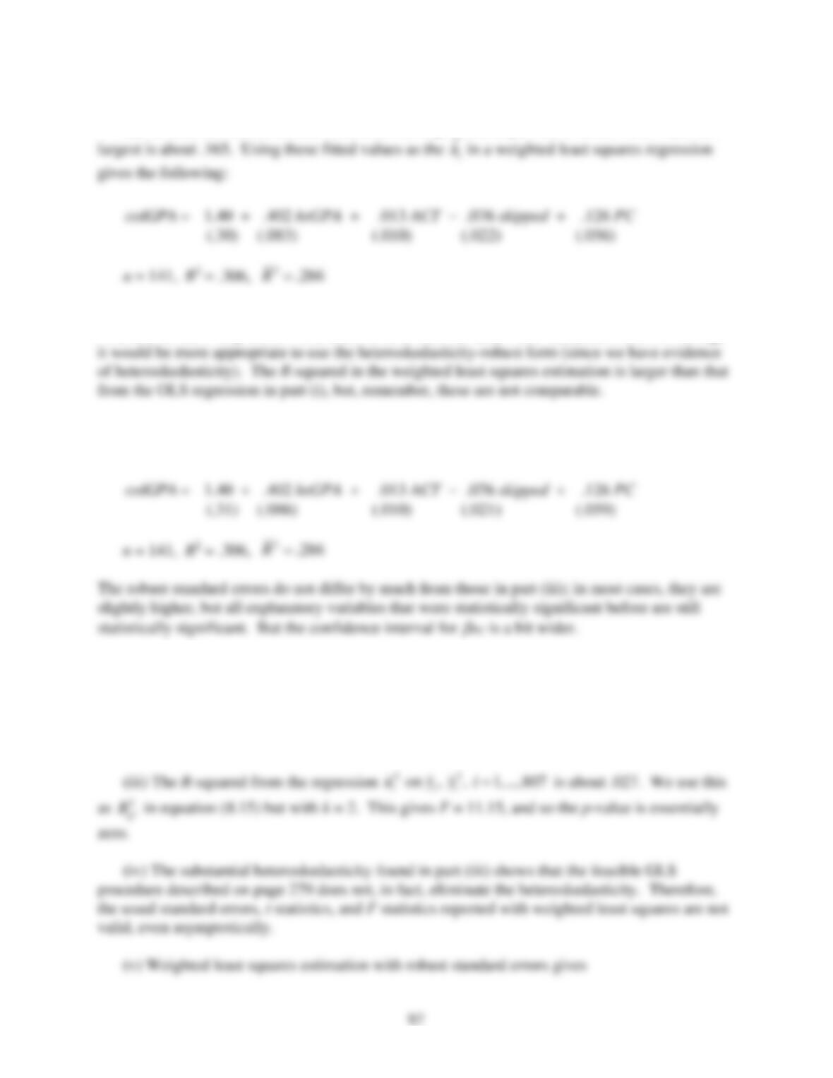
(iii) In fact, the smallest fitted value from the regression in part (ii) is about .027, while the
There is very little difference in the estimated coefficient on PC, and the OLS t statistic and WLS
t statistic are also very close. Note that we have used the usual OLS standard error, even though
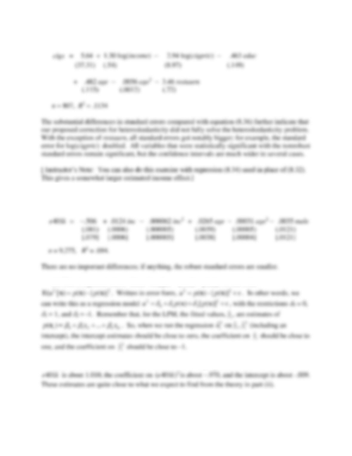
(iv) With robust standard errors – that is, with standard errors that are robust to misspecifying
the function h(x) – the equation is
C8.9 (i) I now get R2 = .0527, but the other estimates seem okay.
(ii) One way to ensure that the unweighted residuals are being provided is to compare them
with the OLS residuals. They will not be the same, of course, but they should not be wildly
different.
98
C8.10 (i) In the following equation, estimated by OLS, the usual standard errors are in () and
the heteroskedasticity-robust standard errors are in []:
(ii) This is a general claim. Since Var(y|x) =
( )[1 ( )]pp−xx
, we can write
(iii) The White F statistic is about 310.32, which is very significant. The coefficient on
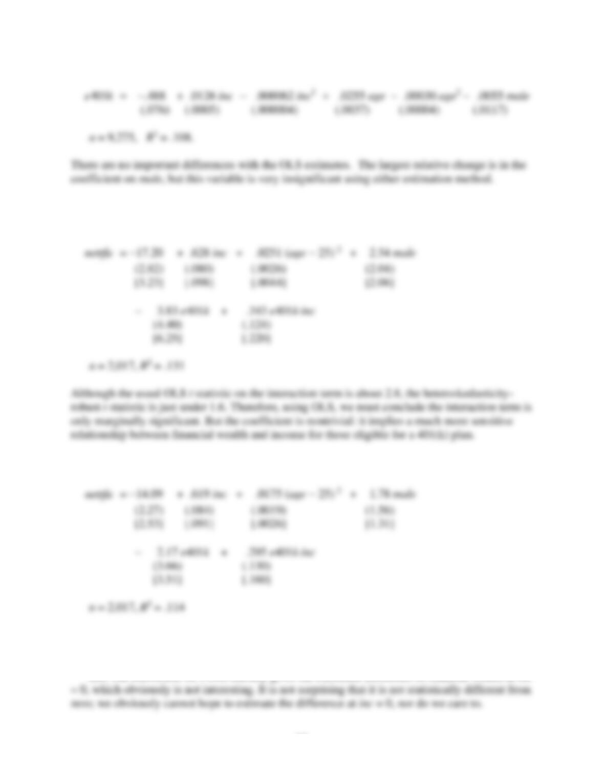
(iv) The smallest fitted value is about .030 and the largest is about .697. The WLS estimates
of the LPM are
99
C8.11 (i) The usual OLS standard errors are in (), the heteroskedasticity-robust standard errors
are in []:
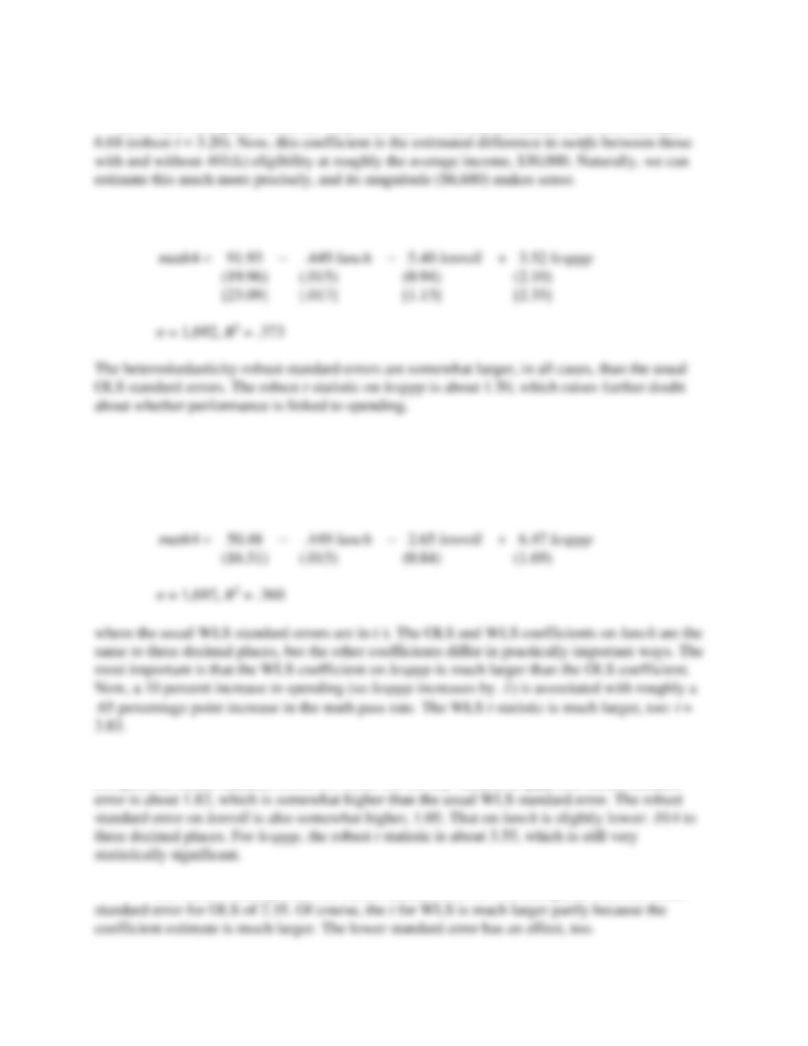
(ii) The WLS estimates, with usual WLS standard errors in () and the robust ones in [], are
The robust t statistic is about 1.84, and so the interaction term is marginally significant (two-
sided p-value is about .066).
(iii) The coefficient on e401k literally gives the estimated difference in financial wealth at inc
100
(iv) When we replace e401kinc with e401k(inc − 30), the coefficient on e401k becomes
C8.12 (i) The estimated equation is
(ii) The value of the F statistic is 132.7, which gives a p-value of zero to at least four
decimal places. Therefore, there is strong evidence of heteroskedasticity.
(iii) The equation estimated by WLS is
(iv) Because our model of heteroskedasticity might be wrong, it is a good idea to
compute the robust standard errors for WLS. On the key variable lexppp, the robust standard
(v) WLS is more precise: its robust standard error is 1.82, compared with the robust
C8.13 (i) The estimated equation with standard errors is
(ii) I used the test command in Stata to obtain both tests. The p-value for the usual
(iii) The test for heteroskedasticity yields and F statistic of 726.11, which is a very large
(iv) Even though we find conclusive evidence of heteroskedasticity, it has only a minor
C8.14 (i) The estimated equation with heteroskedasticity-robust standard errors below
coefficients is
Except for abvavg, the coefficients have the signs we expect. But the coefficient on avbavg has a
very small t statistic; for all practical purposes we can treat it as zero. The coefficients on the
102
(ii) Adding the five interactions produces R2 = .3685. The nonrobust F test for exclusion of
(iii) The coefficients on the
female belavg
and
female abvavg
are about .044 and .082,