194
ADDITIONAL CASE STUDY
8-4 The Decline in the U.S. Saving Rate
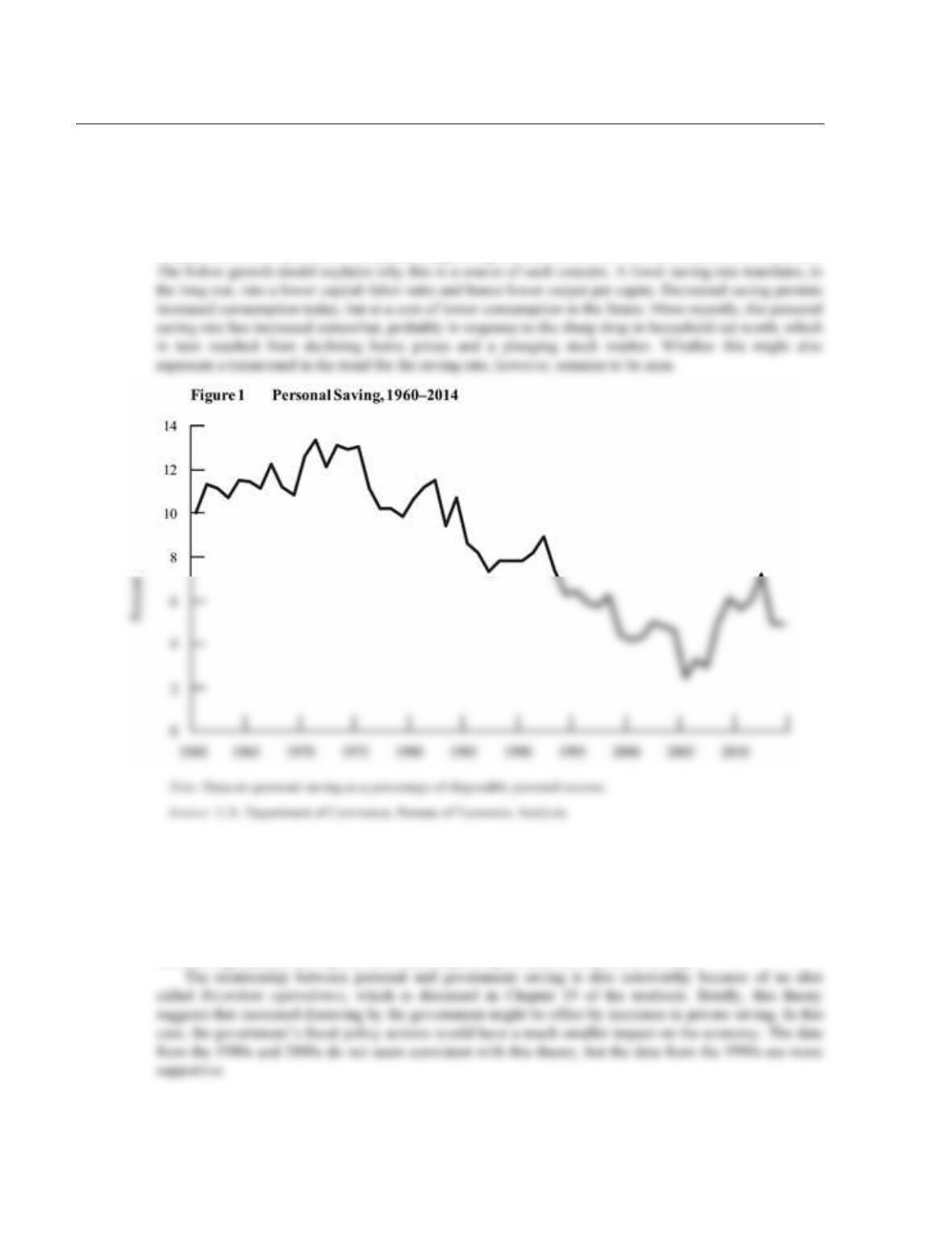
Figure 1 shows personal saving as a percentage of disposable personal income since 1960. From the early
1960s through the mid–1970s, the personal saving rate fluctuated between about 10 percent and 13
percent, and it showed an upward trend. In the late 1970s, however, the saving rate began a decline that
accelerated in the late 1990s and early 2000s, bringing the rate to 2.5 percent by 2005. Many
commentators have pointed to the plummeting saving rate in recent years as a possible cause of concern.
Personal saving is only part of the story. Government saving fell in the 1980s (i.e., the government
deficit increased). Thus, both the government’s fiscal policies and individuals’ consumption/saving
decisions contributed to a fall in national saving, from over 23 percent of national income in the late 1970s
to under 18 percent of national income in the early 1990s. As the government deficit shrank and turned to
surplus, national saving rose to over 20 percent of national income by 2000. Recently, as the budget deficit
has reemerged, public saving has fallen, accompanying the decline in personal saving.
195
ADVANCED TOPIC
8-5 Growth Rates, Logarithms, and Elasticities
Whenever we wish to understand the behavior of variables through time, such as when we are interested in
economic growth or inflation, we need to make use of growth rates. The following is a brief summary of
the mathematics of growth rates and the two related ideas of logarithms and elasticities.
Why We Use Growth Rates
When an economic variable increases through time, it is often misleading simply to consider its absolute
change. For example, an increase in GDP from $5 trillion to $5.1 trillion is surely very different from an
increase in GDP from, say, $1 trillion to $1.1 trillion, even though the increase in each case is $100 billion.
In the first case, the $100 billion increase represents a 2 percent increase; in the second case the same
and so on. Then the change in prices every year would be 10. A bundle of goods that cost $100 in the
initial year would cost $150 five years later. The trouble with simply looking at the year–to–year difference
in the level is that it treats an increase in the price of a good from $10 to $20 in exactly the same way as an
Time
Price Level (P)
Inflation Rate (π)
1
100
2
110
0.1
3
120
0.09
4
130
0.083
5
140
0.077
6
150
0.071
.
.
.
.
.
.
.
.
.
41
500
42
510
0.02
196
Time
P
π
1
100
2
110
0.1
4
133.1
0.1
5
146.4
0.1
6
161.1
0.1
.
.
.
.
.
.
.
.
.
The Mathematics of Growth Rates
Suppose that some variable, x, is growing at the rate gx. Then this means that
xt = (1 + gx)xt–1.
Equivalently, we can rewrite this to show that the growth rate gx is
where ∆ indicates the change between one period and the previous period. In other words, it is the
proportionate change, or percentage change, in the variable.
The growth rate of a product of two variables is approximately equal to the sum of the growth rates of
the variables. Suppose that zt = xtyt. Then,
zt = xtyt
= (1 + gx)xt–1(1 + gy)yt–1
Hence,
(1 + gz) = (1 + gx)(1 + gy)
= 1 + gx + gy + gx gy
⇒ gz = gx + gy + gx gy.
But since gx and gy are usually small numbers, their product will be a very small number, so we can write
gz ≅ gx + gy.
For example, if x is growing at 4 percent and y is growing at 2 percent, then gx = 0.04, gy = 0.02, and gx gy
= 0.0008. Thus,
Logarithms
In the Data Plotter available on the textbook Web site, various transformations of the data are possible.
One of these is to take the logarithm of a series. This is included because economists often find it more
3
121
0.1
197
A logarithm is just a function, like others we use in economics, but with some very useful properties.
In particular, suppose we take the logarithm of our earlier price series.
We find, therefore, that a constant percentage growth rate corresponds to a constant difference in
terms of the logarithm. In general,1
gx = ∆x/x ≅ ∆ln(x).
This is convenient because it allows us to perform many calculations using just addition and subtraction
rather than multiplication and division.
Logarithms have the property that ln(xy) = ln(x) + ln(y).2 We can use this to show, as we did before,
that the growth rate of a product equals the sum of the growth rate of the individual variables. As before,
let zt = xt yt. Then
gz = ∆ln(zt)
= ln(zt) – ln(zt–1)
If a variable is growing at a constant rate through time, this means that its percentage change from
year to year is the same. In log terms,
∆ln(xt) = n.
So
ln(xt) – ln(xt–1) = n
⇒ ln(xt) = ln(xt–1) + n.
With every time period that goes by, ln(x) gets bigger by n. So this means that ln(xt) is a linear function of
time, such as
Time
P
π
ln(P)
1
100
4.6
2
110
0.1
4.7
3
121
0.1
4.8
5
146.4
0.1
5.0
6
161.1
0.1
5.1
.
.
.
.
.
.
.
.
.
.
.
.

198
Elasticities
Many of the parameters in economics are expressed in terms of elasticities. For example, this is true of
many of the parameters in the exercises in the textbook Web site. The idea behind the use of elasticities is
similar to that behind the use of logarithms—they permit us to consider how much one variable changes,
in percentage terms, when another variable changes, also in percentage terms. As an example, we know
that investment depends on the real interest rate. We could simply think about the change in investment for
That is, it tells us the percentage change in y for a given percentage change in x. The elasticity of
investment with respect to the interest rate (or, more concisely, the interest elasticity of investment) is thus
Note that
ADDITIONAL CASE STUDY
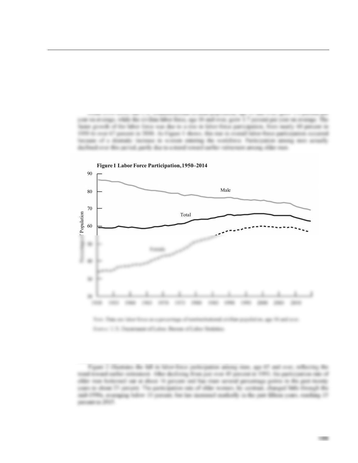
8-6 Labor–Force Participation
The Solow growth model does not distinguish between growth in the population and growth in the labor
force. Instead, it makes the implicit assumption that the labor–force participation rate—the share of the
population in the labor force—is constant through time so that the growth rate of the labor force will be
the same as the growth rate of the population. This assumption is a reasonable one for the purpose of
modeling the process of economic growth. But, for the United States over the period 1950–2000, labor–
force participation increased and contributed importantly to the overall growth of the labor force.
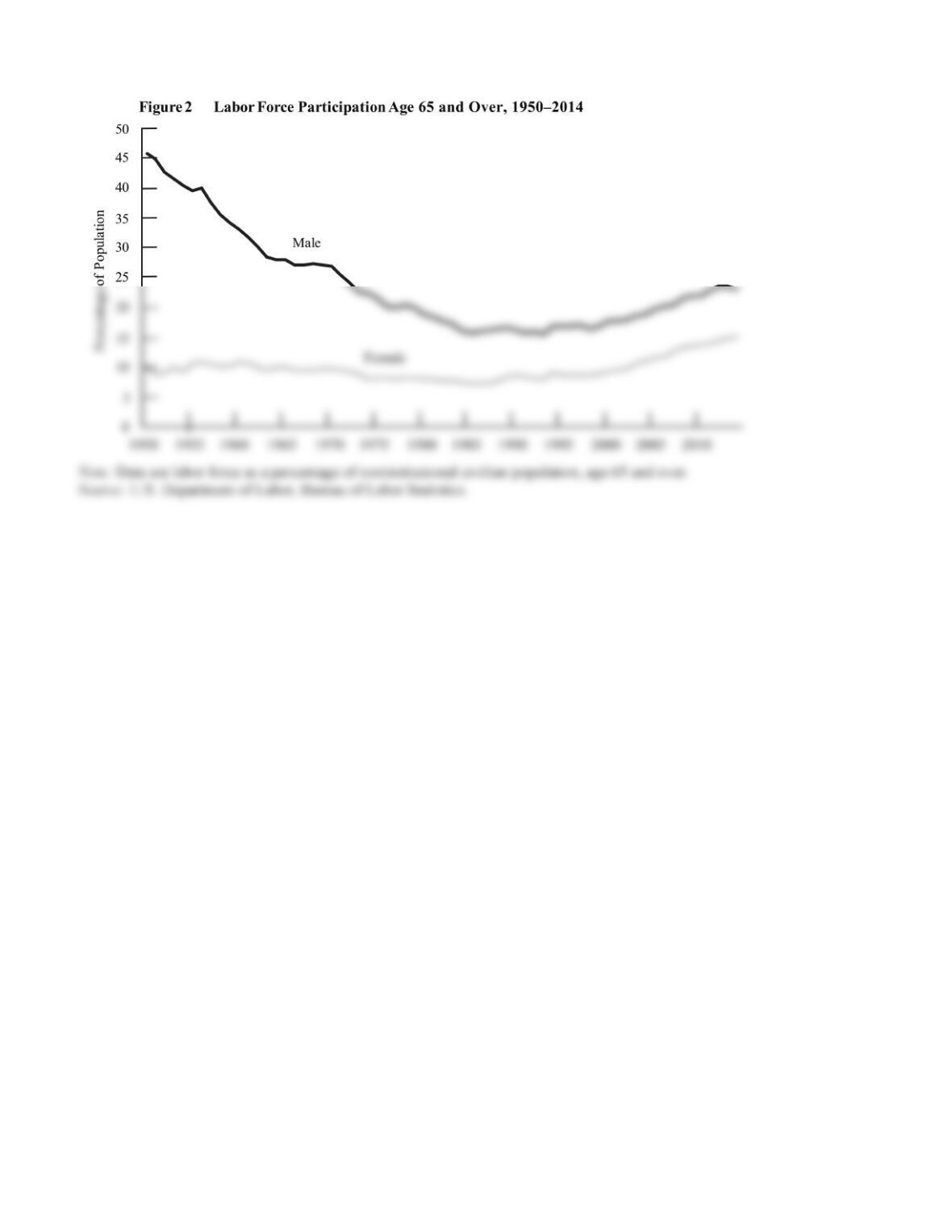
Over the past decade, however, labor force participation plateaued and then declined during and after
the recession of 2008–2009, falling to 63 percent by 2014. Whether the participation rate will increase
once the economy has fully recovered remains an unanswered question.
200
201
ADDITIONAL CASE STUDY
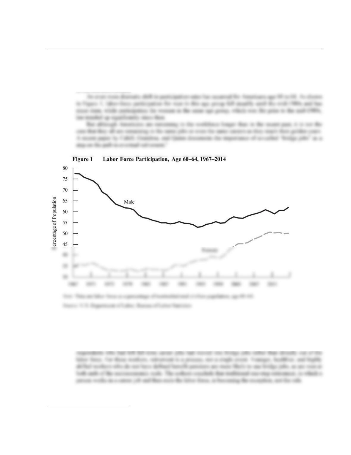
8-7 Bridge Jobs and the Transition to Retirement
As noted in Supplement 8–6, labor–force participation among American men age 65 and over has increased
in the past two decades after declining steadily for much of the post–World War II period, while for older
women, participation has ticked up a bit in recent years after remaining roughly constant through the end
of the twentieth century.
The authors use data from the Health and Retirement Study (HRS) to assess the importance of bridge
jobs among older Americans. These data cover a nationally representative sample of men and women who
were aged 51 to 61 in 1992. The HRS collects information on this sample every two years.2
In their paper, Cahill, Giandrea, and Quinn estimate that between half and two–thirds of the survey
1 Kevin E. Cahill, Michael D. Giandrea, and Joseph F. Quinn, “Retirement Patterns from Career Jobs,” The Gerontologist; October 2006.
2 F.T. Juster and R. Suzman, “An Overview of the Health and Retirement Study,” Journal of Human Resources 30 (Supplement), S7–S56.
202
CASE STUDY EXTENSION
8-8 How Much Variation in Per–Capita Output Is Explained by
s and n?
The case study “Saving and Investment Around the World” showed that cross–country evidence provides
some support for the prediction of the Solow model that countries with higher saving rates have higher
levels of output per capita. The case study “Population Growth Around the World,” in turn, provides
supporting evidence for the prediction that countries with higher population growth rates have lower levels
203
LECTURE SUPPLEMENT
8-9 The Solow Growth Model: An Intuitive Approach—Part One
This supplement presents a more intuitive and less mathematical explanation of the Solow growth model
than appears in the textbook. We carry out all our analysis using the production function found in the
classical model of Chapter 3:
The Accumulation of Capital
Suppose that the labor force and the production function are unchanging. What determines the capital
stock? First, it is important to observe that the capital stock increases as a consequence of investment:
Firms’ spending on new factories and machines increases the stock of capital available in the economy.
Recall from the classical model of Chapter 3 that equilibrium in the loanable–funds market (brought about
by the adjustment of the real interest rate) implies that investment equals national saving. It follows
immediately that the capital stock will increase as a consequence of saving. In the classical model, the
level of saving is fixed and exogenous because the level of output is fixed. But since long–run growth
entails changes in output, it is no longer appropriate to assume that saving is fixed. Rather, it seems
plausible that, as output (or, equivalently, income) increases, so also does saving. We make the simple
assumption that total national saving is proportional to output, so
Total Investment = Total Saving = sY,
sY = δK.
Once at this point, the capital stock will remain there, with new investment each year being just
enough to replace worn–out capital. Such a situation is known as a steady state. This result is perhaps
consoling—if it were not true, then either the capital stock would keep declining through time, and
eventually workers would have no machines to operate, or else it would keep increasing until there were
hundreds of machines and factories for every worker. If the capital stock is below its steady–state level,
total saving exceeds total depreciation and the capital stock increases; the opposite occurs if the capital
stock exceeds its steady–state level.
204
Features of Steady State
We are assuming that the labor force, L, is constant. We have just concluded that, in steady state, K is
constant. It follows immediately that total output, Y, is also constant. (The amount of output available for
consumption by individuals and the government must also be fixed: Since Y = C + I + G, and Y and I are
fixed, it follows that C + G is fixed.) Thus, we have not yet explained long–run growth. Output may grow
Population Growth
Now, let us suppose that the population grows at the rate n (for example, 2 percent per year). Once again,
it turns out that the economy will reach a steady state—in this case, one where the capital stock is growing
at the same rate as the population. Otherwise, the amount of capital relative to the number of workers
would either become arbitrarily large (if the capital stock grew faster than the rate n) or arbitrarily small (if
the capital stock grew more slowly than the rate n). In the steady state, both the population and the capital
stock are growing, but the capital–labor ratio (the number of machines per worker) is constant:
K/L = Constant.
Recall from Chapter 3 that the production function possesses constant returns to scale. By definition,
this means that if K and L are both growing at the rate n, then output is also growing at the rate n. In the
steady state with population growth, output grows at the rate of growth of the population. It follows
immediately that output per person is constant.
There is another important and perhaps less obvious consequence of population growth: Higher
population growth means lower living standards. To see this, suppose that we start with an economy in
steady state with no population growth (so the growth rate of K equals the growth rate of L equals zero).

LECTURE SUPPLEMENT
8-10 Additional Readings
Robert Solow’s book on growth theory is a useful introduction to the topic: R. Solow, Growth Theory