Chapter 8
Endogeneity and Instrumental Variable Estimation
◼ Exercises
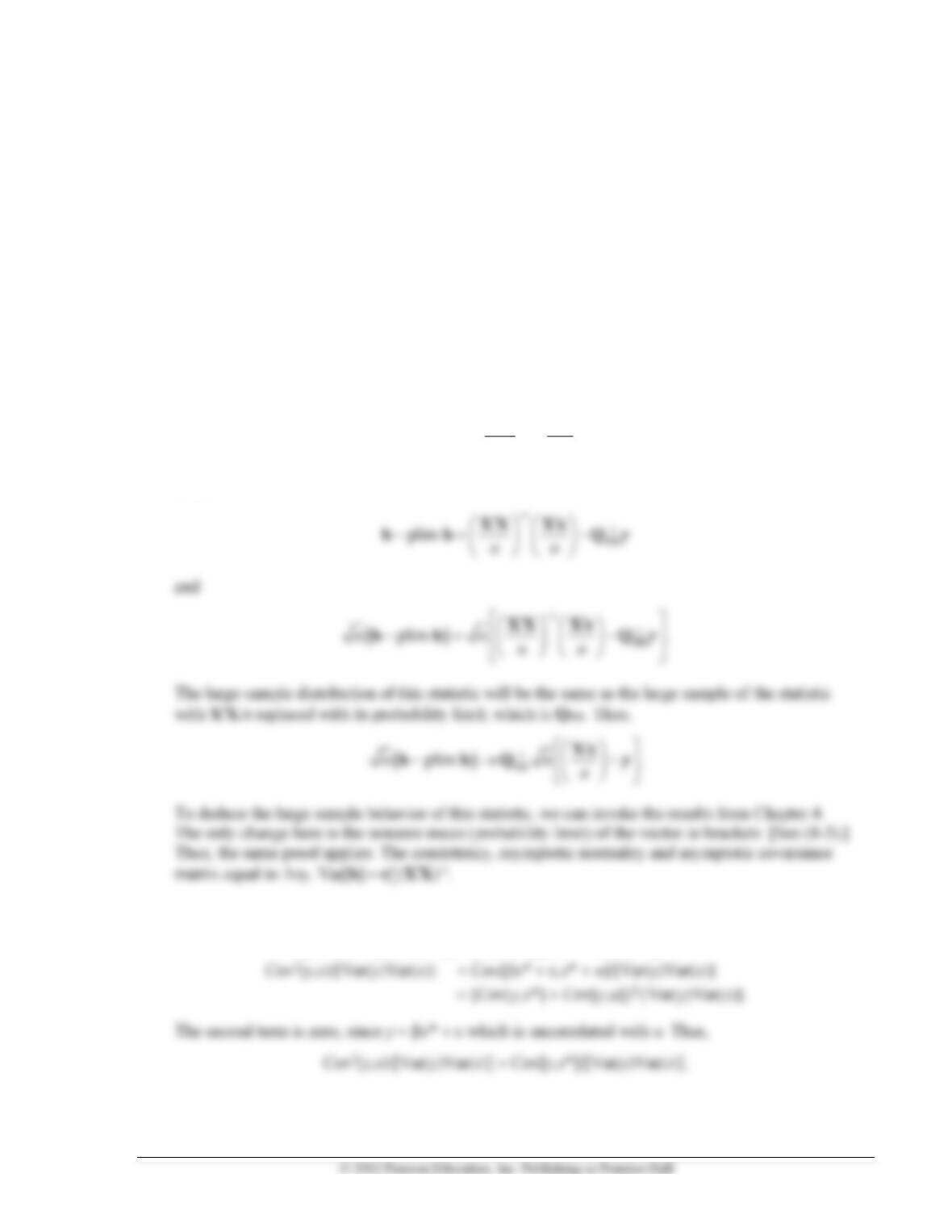
1. There is no need for a separate proof different from the usual for OLS. Formally, however, it follows
from the results at (8-4) that
−
=+
X1
.
nn
XX
b
Then,
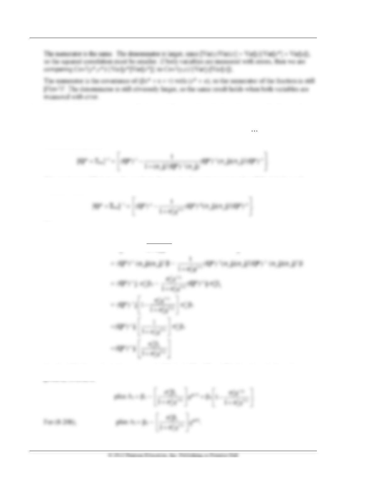
2. A logical solution to this one is simple. For y and x*,
Cov2(y,x*)/[Var(y)Var(x*)] = 2(*2)2/[(2*2 + 2)(*2)]
58 Greene • Econometric Analysis, Seventh Edition
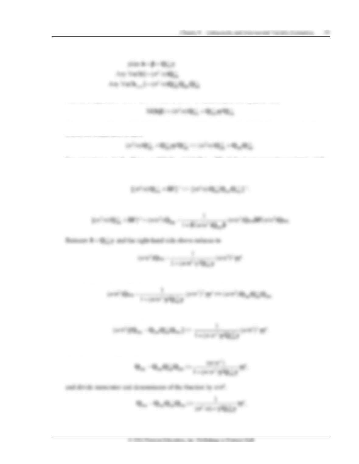
3. We work off (8-19), using repeatedly the result uu = (u j)(u j) where j has a 1 in the first position
and 0 in the remaining K − 1. From (8-19),
plim b = − [Q* + uu]−1uu . The vector is uu equals
2
1
[ 0, ,0] .
u
The inverse matrix is
This can be simplified since the quadratic form in the denominator just picks off the 1,1 diagonal
element. Thus,
Then
[Q* + uu]−1uu =
1 1 1
2 *11
1
( *) ( *) ( )( ) ( *)
1uu
− − −
−
+
Q Q j j Q
( )( )
uu
jj
Finally,
1
( *)−
Q
j equals the first column of
1
( *)−
Q
= [q*11, q*21,…,q*k1]. Therefore, the first element,
given by (8-20a) is
4. To obtain the result, note first:
The mean squared error of the OLS estimator is the variance plus the squared bias,
the mean squared error of the 2SLS estimator equals its variance. For OLS to be more precise than
2SLS, we would have to have
For convenience, let
−
=1,
XX
Q
so M(b|) = (2/n)
1.
−
+
XX
Q
If the mean squared error matrix of the
OLS estimator is smaller than that of the 2SLS estimator, then its inverse is larger. Use (A-66) to do
the inversion. The result would be
Now, use (A-66)
Therefore, if the mean squared error matrix of OLS is smaller, then
Collect the terms, and this implies
Divide both sides by (n/2),
60 Greene • Econometric Analysis, Seventh Edition
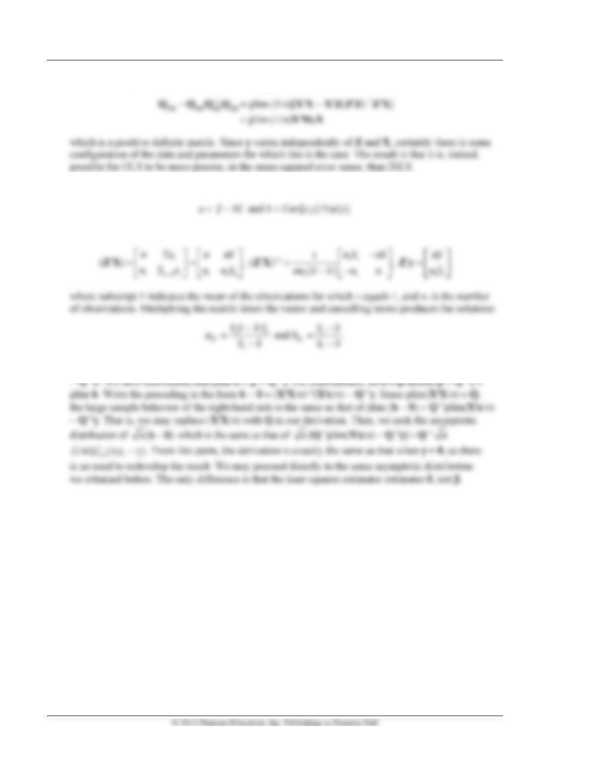
which is the desired result. Is it possible? It is possible, since
5. The matrices are X = [i,x] and Z = [i,z]. For the OLS estimators, we know from Chapter 2 that
For the IV estimator, (ZX)−1Zy, we obtain the result in detail. Given the forms,
6. To obtain the asymptotic distribution, write the result already in hand as b = ( + Q−1) + (XX)−1X
Chapter 8 Endogeneity and Instrumental Variable Estimation 61
Application
The statement of the problem is actually a bit optimistic. Given the way it is stated, it would imply that the
exogenous variables in the “demand” equation would be, in principle, (Ed, Union, Fem), which are also in
the supply equation, plus the remainder, (Exp, Exp2, Occ, Ind, South, SMSA, Blk). The problem is that the
model as stated would not be identified—the supply equation would, but the demand equation would not
be. The way out would be to assume that at least one of (Ed, Union, Fem) does not appear in the demand
equation. Since surely education would, that leaves one or both of Union and Fem. We will assume both of
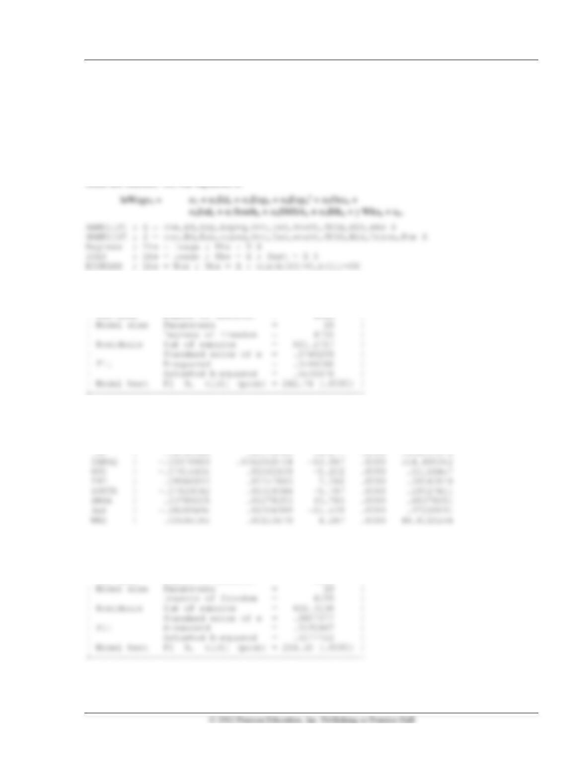
them are omitted. So, our equation is
+—————————————————-+
| Ordinary least squares regression |
| LHS=LWAGE Mean = 6.676346 |
| Standard deviation = .4615122 |
+—————————————————-+
+——–+————–+—————-+——–+——–+———-+
|Variable| Coefficient | Standard Error |b/St.Er.|P[|Z|>z]| Mean of X|
+——–+————–+—————-+——–+——–+———-+
Constant| 5.13171052 .07238152 70.898 .0000
ED | .06112766 .00277226 22.050 .0000 12.8453782
+—————————————————-+
| Two stage least squares regression |
| LHS=LWAGE Mean = 6.676346 |
| Standard deviation = .4615122 |
| WTS=none Number of observs. = 4165 |
62 Greene • Econometric Analysis, Seventh Edition
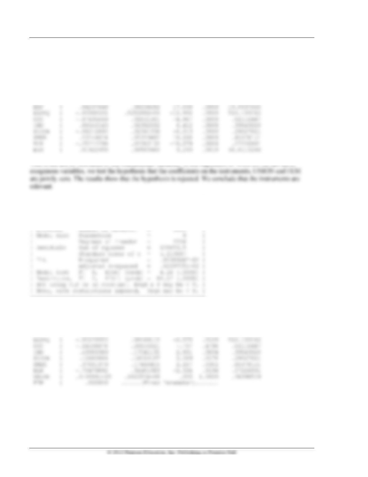
| Instrumental Variables:
|ONE ED EXP EXPSQ OCC IND SOUTH SMSA
|BLK UNION FEM
+——–+————–+—————-+——–+——–+———-+
|Variable| Coefficient | Standard Error |b/St.Er.|P[|Z|>z]| Mean of X|
+——–+————–+—————-+——–+——–+———-+
Constant| 4.46105888 .27680953 16.116 .0000
ED | .06167266 .00283031 21.790 .0000 12.8453782
+—————————————————-+
| Linearly restricted regression |
| Ordinary least squares regression |
| LHS=WKS Mean = 46.81152 |
| Standard deviation = 5.129098 |
+—————————————————-+
+——–+————–+—————-+——–+——–+———-+
|Variable| Coefficient | Standard Error |b/St.Er.|P[|Z|>z]| Mean of X|
+——–+————–+—————-+——–+——–+———-+
Constant| 46.6129896 .67547781 69.007 .0000
ED | -.03787988 .03789322 -1.000 .3175 12.8453782
EXP | .05840099 .03139904 1.860 .0629 19.8537815