08 Case model 9/12/2022 17:17 12/9/2018
Probability
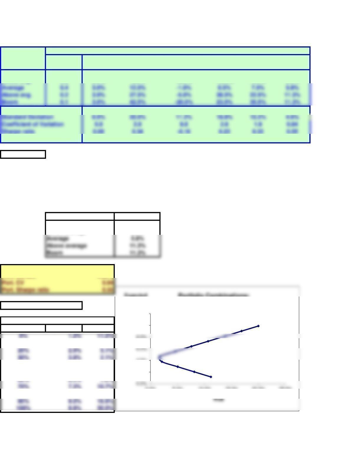
Recession 0.1 3.0% -29.5% 24.5% 3.5% -19.5% -2.5%
Below avg. 0.2 3.0% -9.5% 10.5% -16.5% -5.5% 0.5%
Expected Return 3.0% 9.9% 1.2% 7.3% 8.0% 5.5%
Beta 0.00 1.31 -0.50 0.88 1.00 0.41
PART F
weight in High Tech 50%
weight in Collections 50%
State of the economy Port. return
Recession -2.5%
Below average 0.5%
Port. Sharpe ratio 0.55
Portfolio return 5.53%
Port. std dev 4.62%
Correlation = -0.9885
% in HT Exp. ret. Std. dev.
10% 2.0% 8.1%
40% 4.7% 1.7%
50% 5.5% 4.5%
80% 8.2% 13.8%
Chapter 8. Risk and Rates of Return
Returns on Alternative Investments
T-Bills
Market
portfolio
High Tech/Collections Portfolio
2-Stock
Portfolio
State of the
Economy
High Tech
Collections
U.S.
Rubber*
This spreadsheet model is designed to be used in conjunction with the chapter’s integrated case and the related
PowerPoint slide presentation.
Suppose you created a 2-stock portfolio by investing $50,000 in High Tech and $50,000 in Collections. (1)
Calculate the expected return, the standard deviation, the coefficient of variation, and the Sharpe ratio for this
portfolio, and fill in the appropriate blanks in the table.
2.0%
4.0%
8.0%
10.0%
12.0%
0.0% 5.0% 10.0% 15.0% 20.0% 25.0%
Expected
return
Portfolio Combinations:
HT and Collections
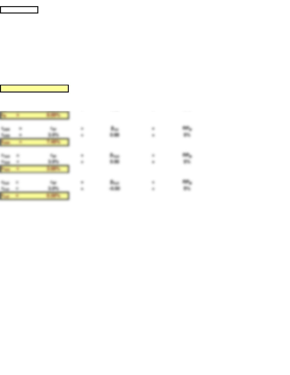
PART J
Risk-free rate 3.0% Risk-free rate 3.0%
RPM5.0% RPM5.0%
Beta 1CAPM 8.0%
rHT = rRF +βHT ×RPM
rHT = 3.0% +1.31 ×5%
rHT = 9.55%
rM = rRF +βM×RPM
rM = 3.0% +1.00 ×5%
The yield curve is currently flat; that is, long-term Treasury bonds also have a 3.0% yield. Consequently, Merrill
Finch assumes that the risk-free rate is 3.0%. (1) Write out
the SML equation, use it to calculate the required rate of return on each alternative, and graph the relationship
between the expected and required rates of return.
rM = 8.00%
rUSR = rRF +βUS ×RPM
rUSR = 3.0% +0.88 ×5%
rUSR = 7.40%
rTbill = rRF +βTbill ×RPM
rTbill = 3.0% +0.00 ×5%
rTbill = 3.00%
rColl = rRF +βColl ×RPM
rColl = 3.0% + -0.50 × 5%
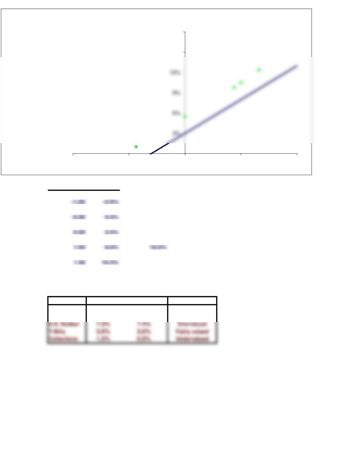
Beta
rs
8.0%
-0.87 -1.4% 1.0%
0.00 3.0% 5.5%
0.88 7.4% 9.8%
1.32 9.6% 12.4%
2.00 13.0%
Security Exp. Ret. Req. Ret. Conclusion
High Tech 17.4% 1.30
9.9% 9.6% Undervalued
Market 8.0% 8.0% Fairly valued
(2) How do the expected rates of return compare with the required rates of return?
0%
15%
18%
-2.00 -1.00 0.00 1.00 2.00
Required and
Expected Returns
Beta
βp = wHT xβHT + wColl xβColl
βp = 0.5 x1.31 +0.5 x -0.50
βp = 0.405
βp = wHT xβHT + wUSR xβUSR
βp = 0.5 x1.31 +0.5 x0.88
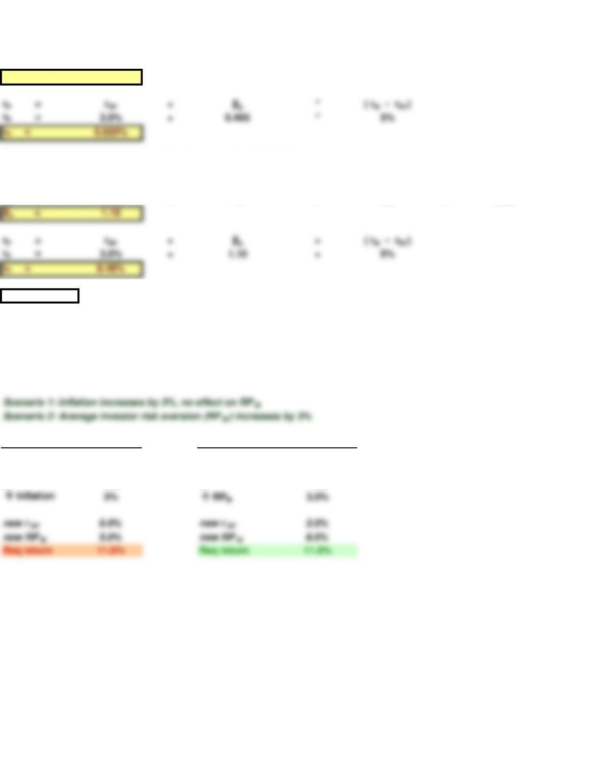
PART K
old rRF 3.0% old rRF 3.0%
old RPM5.0% old RPM5.0%
bi1.00 bi1.00
Scenario 1
Scenario 2
(1) Suppose investors raised their inflation expectations by 3 percentage points over current estimates as
reflected in the 3.0% risk-free rate. What effect would higher inflation have on the SML and on the returns
required on high- and low-risk securities?
(2) Suppose instead that investors’ risk aversion increased enough to cause the market risk premium to increase
by 3 percentage points. (Inflation remains constant.) What effect would this have on the SML and on returns of
high- and low-risk securities?
(4) What would be the market risk and the required return of a 50-50 portfolio of High Tech and Collections?
For a portfolio consisting of 50% High Tech and 50% U.S. Rubber?
rP = rRF +βp* ( rM – rRF)
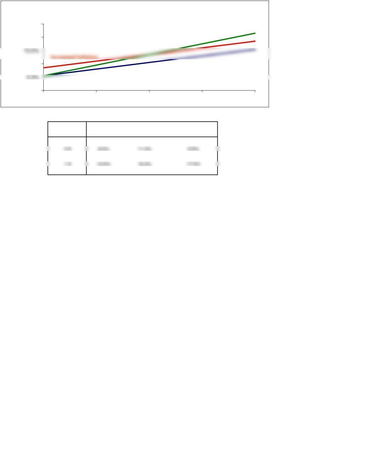
DATA TABLE USED TO MAKE SML GRAPH
Original Scenario 1 Scenario 2
Beta 8.0% 11.0% 11.00%
0 5.5% 8.5% 5.5%
1 10.5% 13.5% 13.5%
2 15.5% 18.5% 21.5%
0.0%
10.0%
20.0%
25.0%
0 0.5 1 1.5 2
Required return
Beta
Changes in the SML
Original Scenario
Increased Risk Aversion