
08 Chapter model 12/12/2018
STAND-ALONE RISK (Section 8-2)
PROBABILITY DISTRIBUTIONS: CALCULATING EXPECTED RETURN
Table 8.1 Probability Distributions and Expected Returns
Rate of Rate of
Economy, Probability Return Probability Return
Which of This if This of This if This
Affects Demand Demand Product Demand Demand Product
Demand Occurring Occurs
(2) × (3) Occurring Occurs (5) × (6)
(1) (2) (3) (4) (5) (6) (7)
Strong 0.30 80% 24% 0.30 15% 4.5%
PROBABILITY DISTRIBUTIONS: CALCULATING STANDARD DEVIATION
U.S. Water
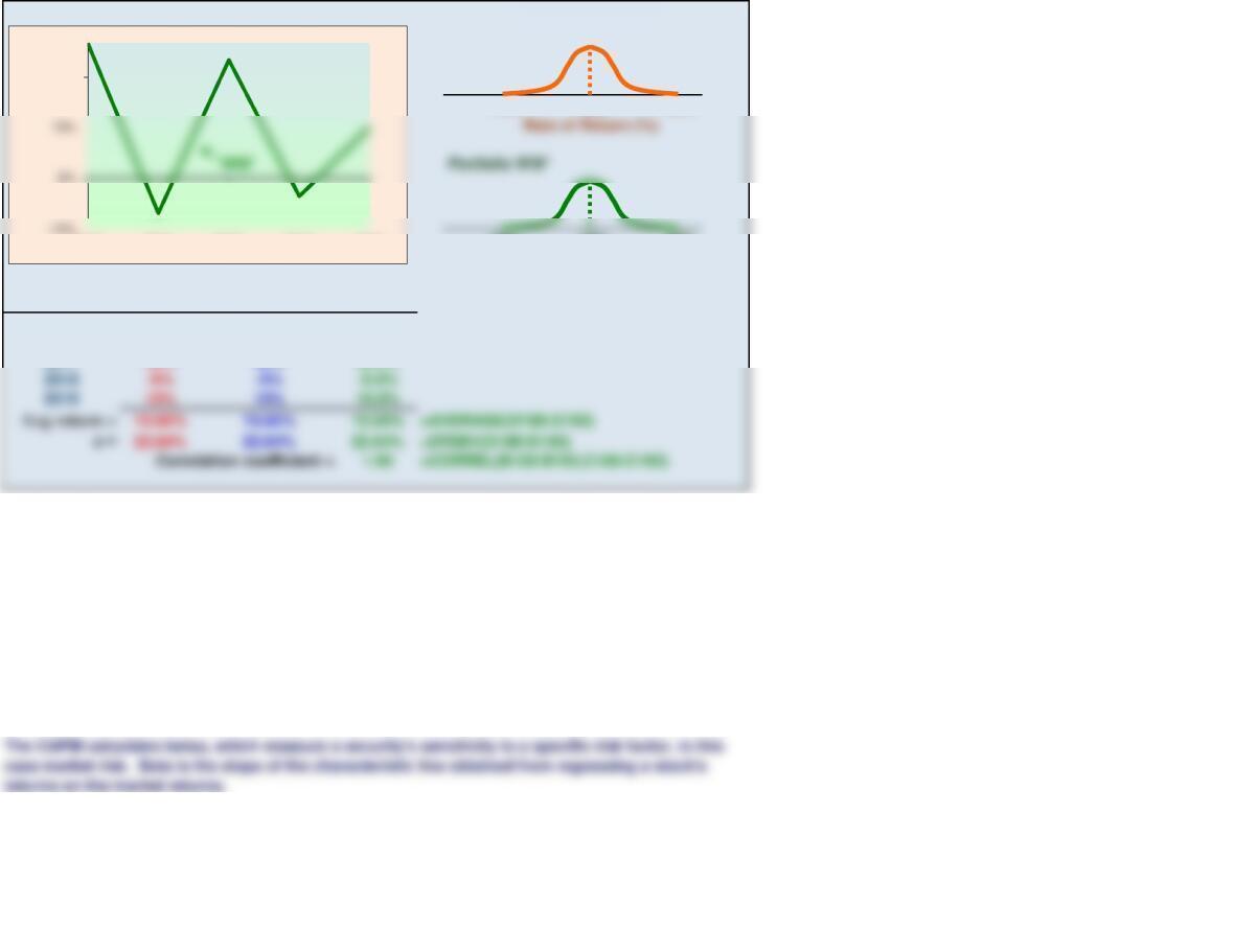
Standard deviation measures the variability of a set of observations and is calculated by finding the
square root of a sum of squared deviations. Sound confusing? The charts below calculate
9/12/2022 15:40
In explaining stand-alone risk, this model introduces probability distributions and the calculation of
expected returns, standard deviations, and coefficients of variation.
The relationship between risk and return is a fundamental axiom in finance. Generally speaking, it
is totally logical to assume that investors are only willing to assume additional risk if they are
Chapter 8. Risk and Rates of Return
The probability distribution is a listing of all possible outcomes and the corresponding probability.
The expected return is calculated by multiplying the possible returns by their corresponding
probabilities.
Martin Products
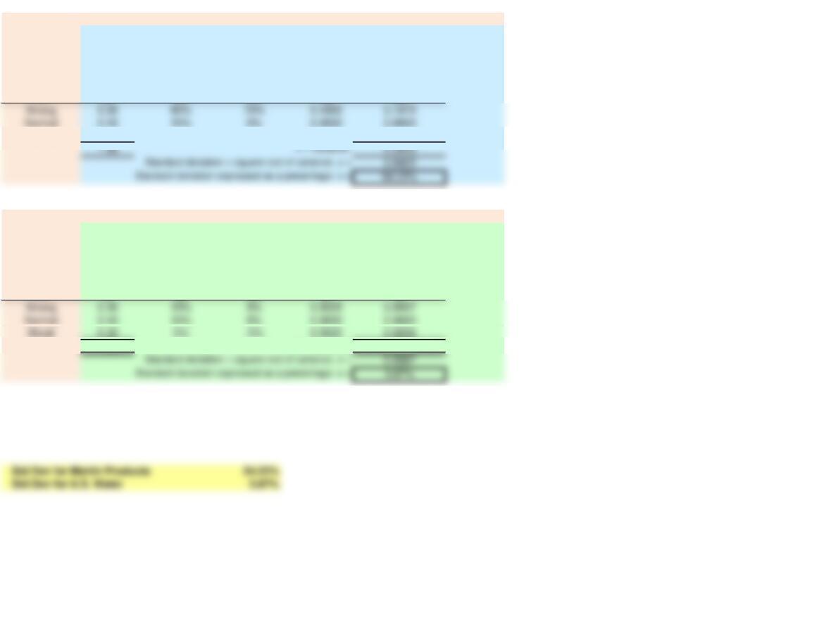
Table 8.2 Calculating Martin Products’ Standard Deviation
Rate of Deviation:
Economy, Probability Return
Actual –
Which of This if This 10% Squared
Affects Demand Demand Expected Deviation Deviation
Demand Occurring Occurs Return Squared
× Prob.
(1) (2) (3) (4) (5) (6)
Weak 0.30 -60% -70% 0.4900 0.1470
1.00 Σ = Variance: 0.2940
Calculating U.S. Water’s Standard Deviation
Rate of Deviation:
Economy, Probability Return
Actual –
Which of This if This 10% Squared
Affects Demand Demand Expected Deviation Deviation
Demand Occurring Occurs Return Squared
× Prob.
(1) (2) (3) (4) (5) (6)
1.00 Σ = Variance: 0.0015
When you calculate standard deviations from expected data in which all states of the world are
accounted for (where the sum of probabilities is 1), you are calculating a population standard
deviation (hence the use of Excel’s population standard deviation function, STDEVP).
Alternatively, you can use Excel’s STDEVP function by entering each return into the formula in the
same proportion as its probability. For instance, Strong demand occurs with a 30% probability, so
enter it three times. Notice this only works if the probabilities are nice, round numbers.
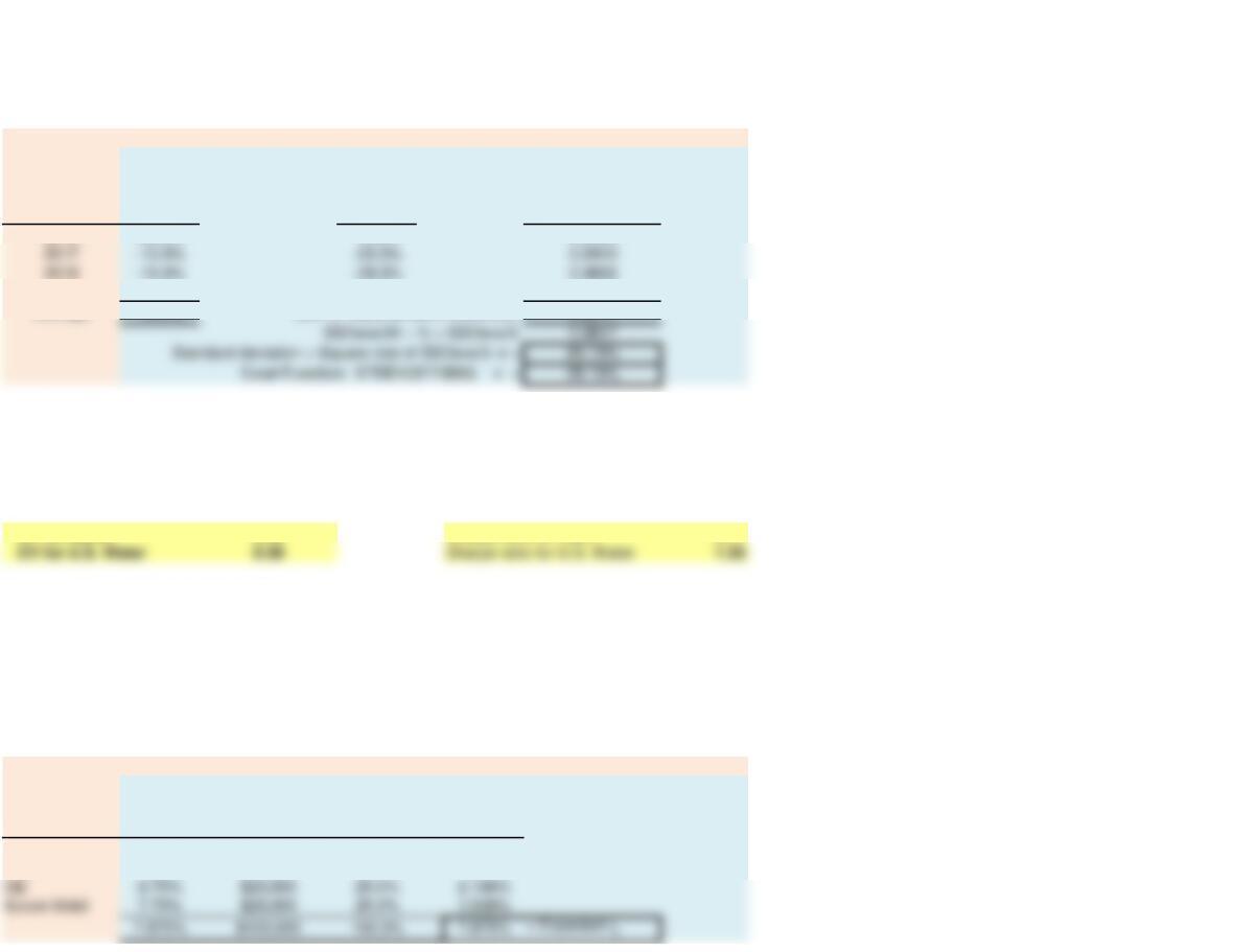
SAMPLE STANDARD DEVIATION CALCULATION
Table 8.3 Finding s Based on Historical Data
Deviation
from Squared
Year Return Average Deviation
(1) (2) (3) (4)
2016 30.0% 19.8% 0.0390
2019 40.0% 29.8% 0.0885
Average 10.3% 0.2541
COEFFICIENT OF VARIATION
Risk-free Rate 4.00%
CV for Martin 5.42 Sharpe ratio for Martin 0.11
CV for U.S. Water 0.39 Sharpe ratio for U.S. Water 1.55
RISK IN A PORTFOLIO CONTEXT (Section 8-3)
PORTFOLIO EXPECTED RETURN
Table 8.4 Expected Return on a Portfolio
Expected Dollars Percent of Product:
Stock Return Invested
Total (wi)(2) × (4)
(1) (2) (3) (4) (5)
Microsoft 7.75% $25,000 25.0% 1.938%
IBM 7.25% $25,000 25.0% 1.813%
More often in finance, you are dealing with a sample of historical data. In this case you need to
calculate a sample standard deviation. This process is outlined in the table below for a fictional
stock, and the Excel shortcut is also shown
Sum of Squared Devs (SSDevs):
Since stocks should be held in conjunction with well-diversified portfolios, it is important to analyze
them in terms of portfolio risk and return.
A problem sometimes arises when comparing standard deviations of different securities. If they
have different expected returns, you may not be able to compare them. The coefficient of variation
shows risk per unit of expected return.
A portfolio’s expected return is merely the weighted average of expected returns of the portfolio’s
components.
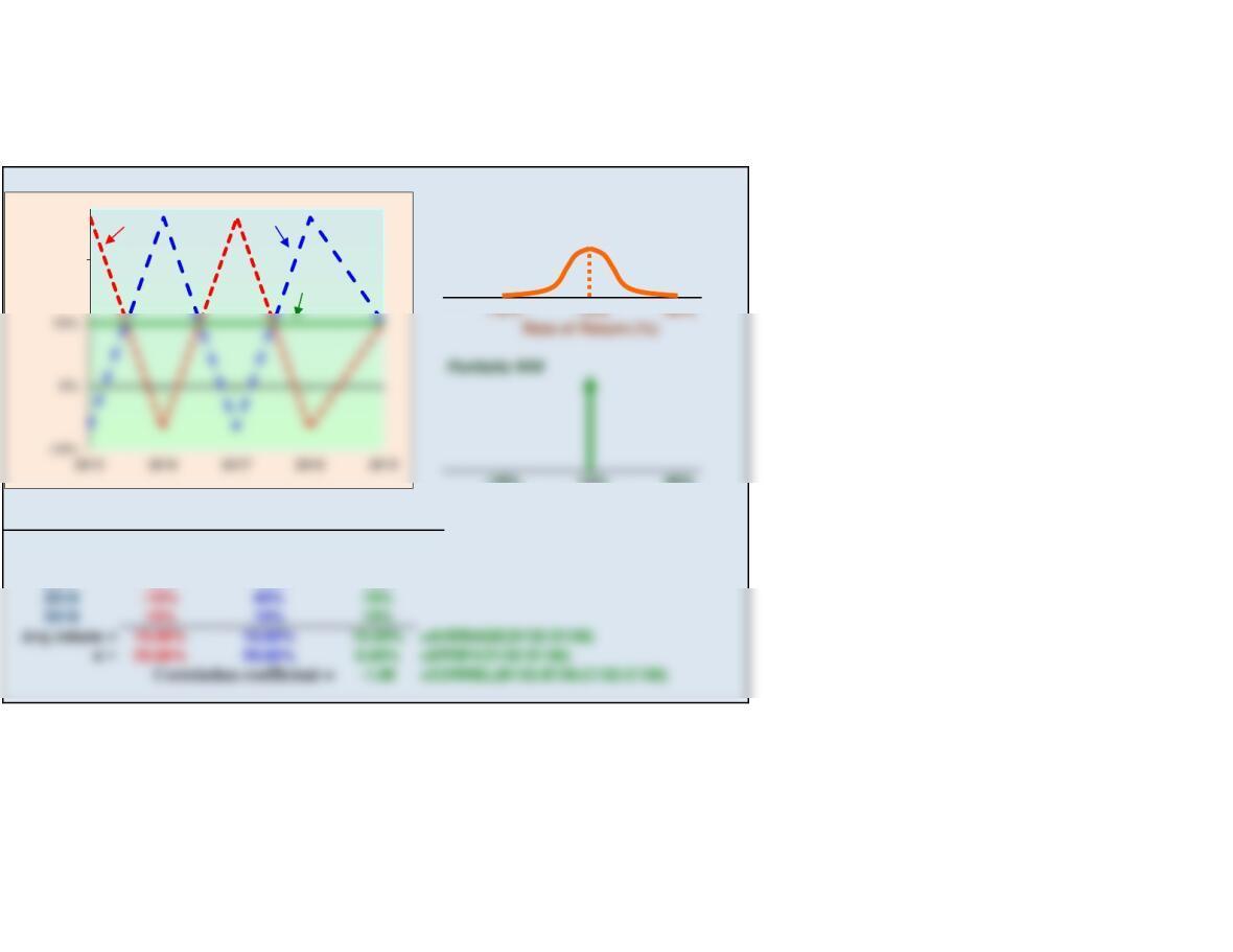
PORTFOLIO RISK
Stocks W and M, held separately
-10% 15% 40%
Rate of Return (%)
Year Stock W Stock M Portfolio WM
2015 40% -10% 15%
2016 -10% 40% 15%
2017 40% -10% 15%
2018 -10% 40% 15%
2019 15% 15% 15%
Figure 8.4 Returns with Perfect Negative Correlation, ρ = -1.0
CONCLUSION: When two stocks are perfectly negatively correlated, diversification is its strongest,
and in this case the portfolio return is a certain (no risk) 15%. Of course, this situation is very rare.
Portfolios of stocks are created to diversify investors from unnecessary risk. The diversifiable, or
idiosyncratic, risk is eliminated as more stocks are added. Diversification effects are strongest
when combining uncorrelated assets. The next few tables (and corresponding graphs) illustrate
how creating two-stock portfolios with different correlations between stocks affects the expected
return and risk of various fictional portfolios.
30%
Rate of
Return
W
M
WM
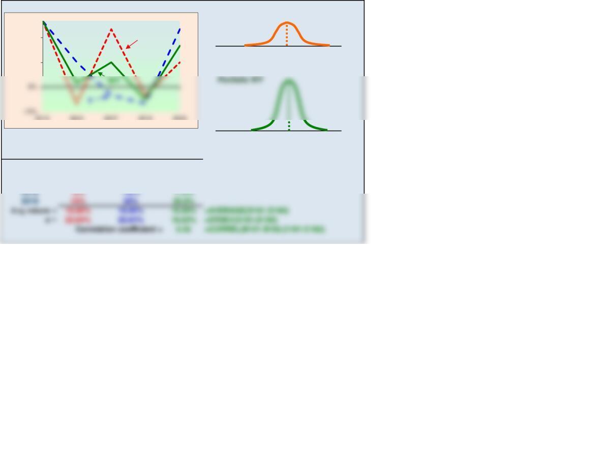
Figure 8.5 Returns with Partial Correlation, ρ = + 0.35
Stocks W and Y, held separately
-10% 15% 40%
Rate of Return (%)
-10% 15% 40%
Rate of Return (%)
Year Stock W Stock Y Portfolio WY
2015 40% 40% 40.0%
2016 -10% 15% 2.5%
2017 35% -5% 15.0%
2019 15% 35% 25.0%
CONCLUSION: In the case where two stocks are somewhat correlated, diversification is effective in
lowering portfolio risk. Here, the portfolio return is an average of the stock returns and risk is
reduced from 22.64% per stock to 18.62% for the portfolio. If more similarly correlated stocks were
added, risk would continue to fall.
15%
30%
2015 2016 2017 2018 2019
Rate of
Return
W
Returns with Perfect Positive Correlation, ρ = + 1.0
Stocks W and W’, held separately
-10% 15% 40%
-10% 15% 40%
Rate of Return (%)
Year Stock W Stock W’ Portfolio WW’
2015 40% 40% 40.0%
2016 -10% -10% -10.0%
2017 35% 35% 35.0%
2019 15% 15% 15.0%
MARKET RISK AND BETA
Diversification can eliminate a lot of risk, but the risk that cannot be diversified away is called
market risk. This is the risk that should be priced in expected returns. An asset pricing model that
does focus on market risk is the Capital Asset Pricing Model (CAPM).
CONCLUSION: When two stocks are perfectly positively correlated, diversification has no effect and
the portfolio’s risk is a weighted average of its stock’s risk. Note, in this graph only the portfolio
returns are visible, but realize that the stock returns follow the same path. In other words, the line
shown is actually all three lines at once.
30%
2015 2016 2017 2018 2019
Rate of
Return
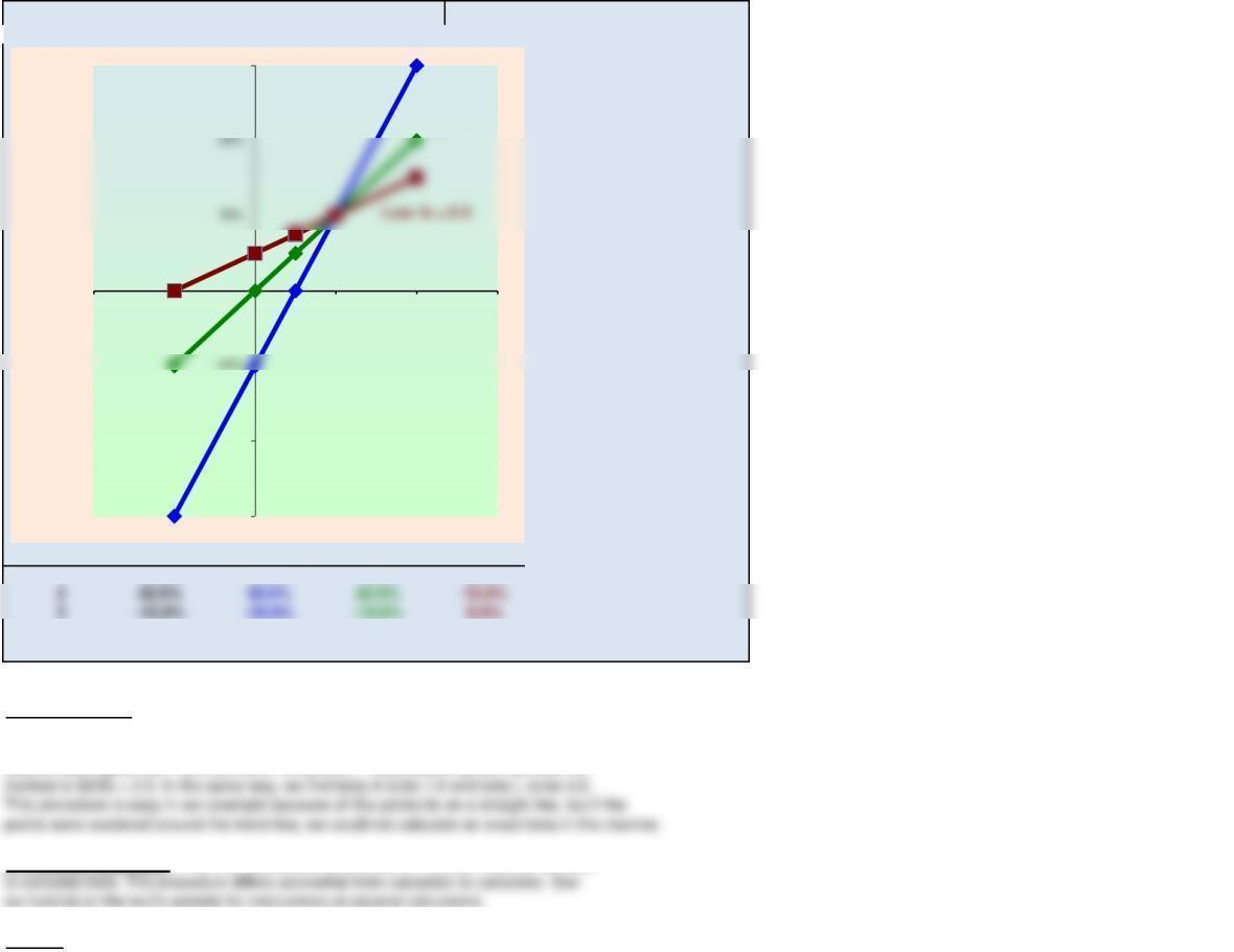
Figure 8.7 Betas: Relative Volatility of Stocks H, A, and L
Year
rMrHrArL
110.0% 10.0% 10.0% 10.0%
40.0% -10.0% 0.0% 5.0%
55.0% 0.0% 5.0% 7.5%
Calculating beta:
1. Rise-Over-Run. Divide the vertical axis change that results from a given change on
the horizontal axis, i.e., the change in the stock’s return divided by the change in the
market return. For Stock H, when the Market rises from -10% to +20%, or by 30%, the
stock’s return goes from -30% to +30%, or by 60%. Thus, beta H by the rise-over-run
2. Financial Calculator. Financial calculators have a built-in function that can be used
3. Excel. Excel’s Slope function can be used to calculate betas. Here are the functions
-30%
-20%
0%
30%
-20% -10% 0% 10% 20% 30%
Return on
Stocks
Return on Market
High: b = 2.0
Average: b = 1.0
220.0% 30.0% 20.0% 15.0%

for our three stocks:
BetaA1.0 =SLOPE(D235:D239,B235:B239)
THE RELATIONSHIP BETWEEN RISK AND RATES OF RETURN (Section 8-4)
SECURITY MARKET LINE
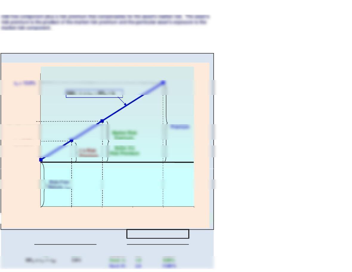
Figure 8.8 The Security Market Line (SML)
The SML shows the relationship between the stock’s beta and its required return, as predicted by
the CAPM.
The CAPM posits that only market risk matters and an asset’s required return should consist of a
rRF = 3.0%
rL= 5.5%
r
A
= r
M
= 8.0%
Required Rate
of Return
RPM. Also
H’s Risk
SML: ri = rRF + (RPM)bi
Beta
ri
rRF 3.0% Riskless asset: 0.0 3.00%
rM8.0% Stock L: 0.5 5.50%
Key Inputs
0 0.5 1 1.5 2 2.5
Beta Coefficient
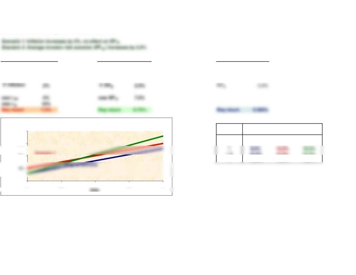
Changing market conditions
Scenario 1 Scenario 2 Original Scenario
old rRF 3% rRF 3% rRF 3.0%
old rM8% old rM8% rM8.0%
bi0.5 bi0.5 bi0.5
DATA TABLE USED TO MAKE SML GRAPH
Original Scenario 1 Scenario 2
Beta
5.5% 7.5% 6.75%
03.0% 5.0% 3.0%
0.5 5.5% 7.5% 6.8%
18.0% 10.0% 10.5%
1.5 10.5% 12.5% 14.3%
213.0% 15.0% 18.0%
Here, two market-affecting scenarios are considered.
The SML prices any asset in the market. So all assets lie somewhere on the SML (in terms of beta
and required return).
10%
15%
20%
Required Return Changes in the SML
Scenario 2
0%
0 0.5 1 1.5 2
SECTION 8-2 12/12/2018
SOLUTIONS TO SELF-TEST QUESTIONS
Probability
Return Prob x Ret.
50% 20% 10.0%
6. An investment has a 50% chance of producing a 20% return, a 25% chance of producing an
8% return, and a 25% chance of producing a -12% return. What is its expected return?
SECTION 8-3 12/12/2018
SOLUTIONS TO SELF-TEST QUESTIONS
Stock
Investment Beta
X$25,000 1.5
7. An investor has a 2-stock portfolio with $25,000 invested in Stock X and $50,000 invested in
Stock Y. X’s beta is 1.50 and Y’s beta is 0.60. What is the beta of the investor’s portfolio?
SECTION 8-4 12/12/2018
SOLUTIONS TO SELF-TEST QUESTIONS
Beta 1.2
Risk-free rate 4.5%
7. A stock has a beta of 1.2. Assume that the risk-free rate is 4.5% and the market risk
premium is 5%. What is the stock’s required rate of return?
Year
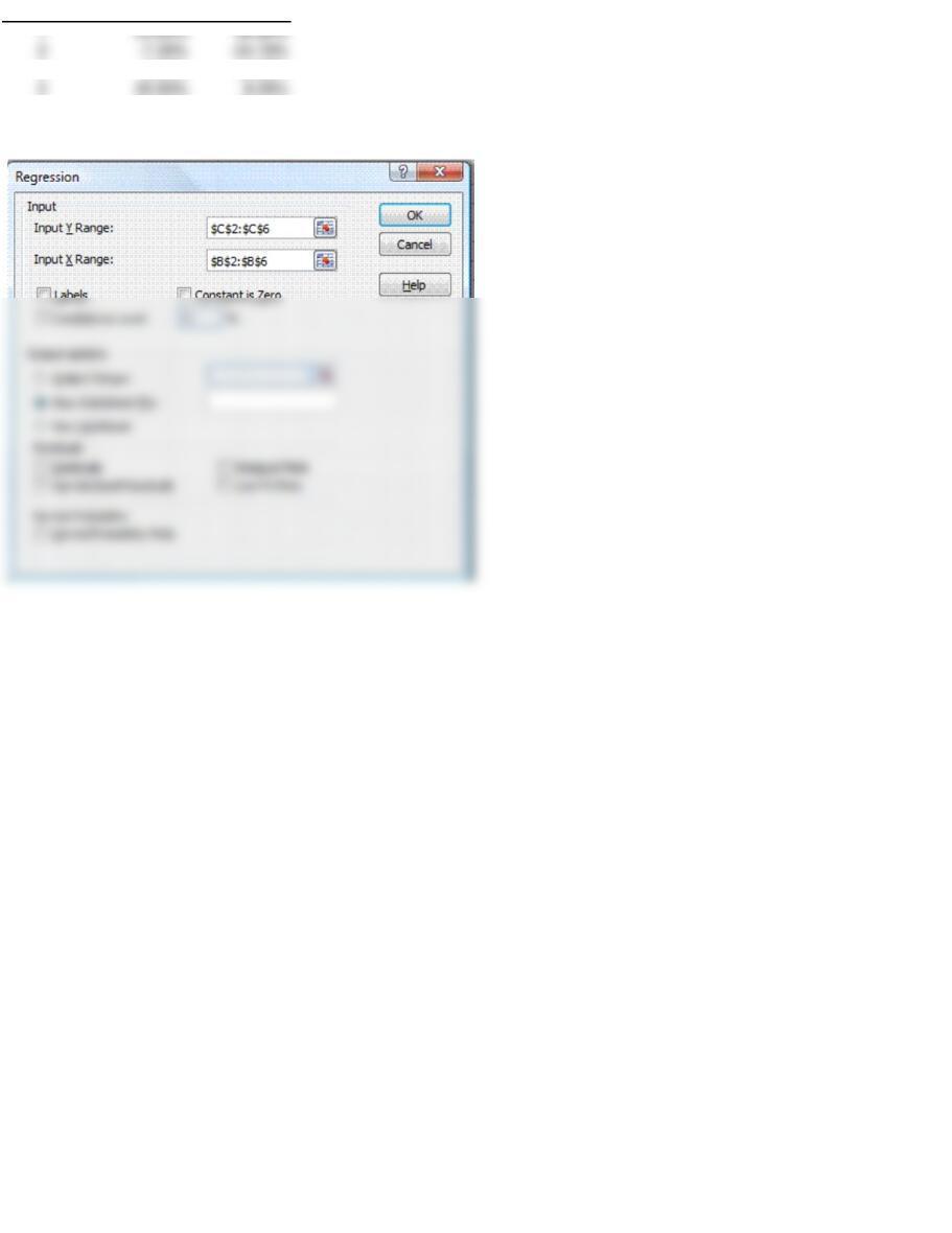
Market (rM) Stock (rJ)12/12/2018
36.60% 12.30%
530.60% 40.10%
Dialog Box to Set Up Regression Analysis

SUMMARY OUTPUT
Regression Statistics
Multiple R 0.91339175
ANOVA
df SS MS F Significance F
Regression 1 0.234979562 0.23498 15.103 0.030195958
Residual 3 0.046674438 0.01556
Total 4 0.281654
Coefficients Standard Error t Stat P-value Lower 95% Upper 95% Lower 95.0% Upper 95.0%