Basic Econometrics, Gujarati and Porter
71
CHAPTER 8:
MULTIPLE REGRESSION ANALYSIS:
THE PROBLEM OF INFERENCE
8.1 (a) In the first model, where sales is a linear function of time, the
(b) The simplest thing to do is plot Y against time. If the resulting
(d) Look up the web sites of several car manufacturers, or Motor
8.2
( ) /
/( )
new old
new
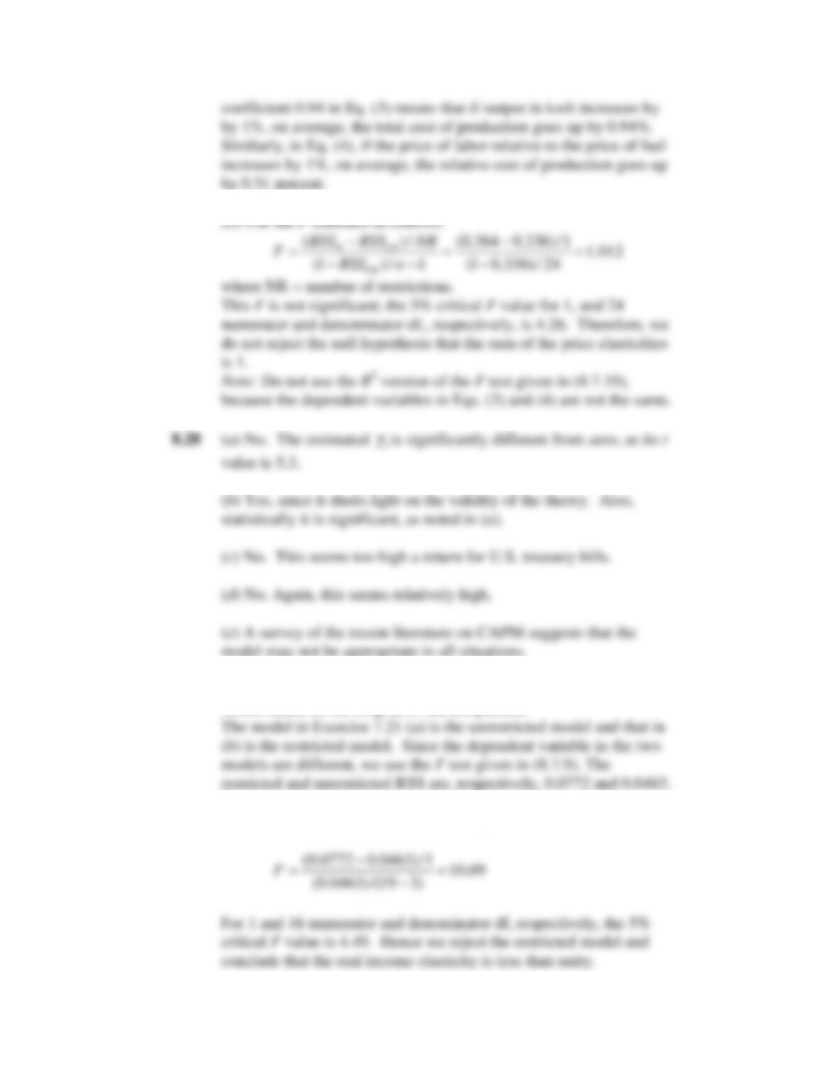
ESS ESS NR
FRSS n k
−
=−
(8.5.16)
8.3
This is a definitional issue. As noted in the chapter, the unrestricted
8.4
In OLS estimation we minimize the RSS without putting any
restrictions on the estimators. Hence, the RSS in this case represents
Basic Econometrics, Gujarati and Porter
72
1
8.5
(a) Let the coefficient of log K be
*
2 3
( 1)
β β β
= + −
. Test the null
(
b
) If we define the ratio (Y/K) as the output/capital ratio, a measure
(
c
) Although the analysis is symmetrical, assuming constant returns
For regression (8.2.1), n=64, k = 3. Therefore,
8.7
Since regression (2) is a restricted form of (1), we can first
calculate the
F
ratio given in (8.5.18):
Basic Econometrics, Gujarati and Porter
73
8.8
The first model can alternatively be written as:
which, after collecting terms, can be written as:
8.9
The best way to understand this term is to find out the rate of change
of Y (consumption expenditure) with respect to X
and X
, which is:
8.10
Recalling the relationship between the t and F distributions, we
2n-k.
8.11
1. Unlikely, except in the case of very high multicollinearity.
Empirical Exercises
8.12
Refer to the regression results given in Exercise 7.21.
(b)
Individually, the income elasticity is significant in both cases,
(c)
Using the R
2
version of the F test given in (8.5.11), the F values
(d)
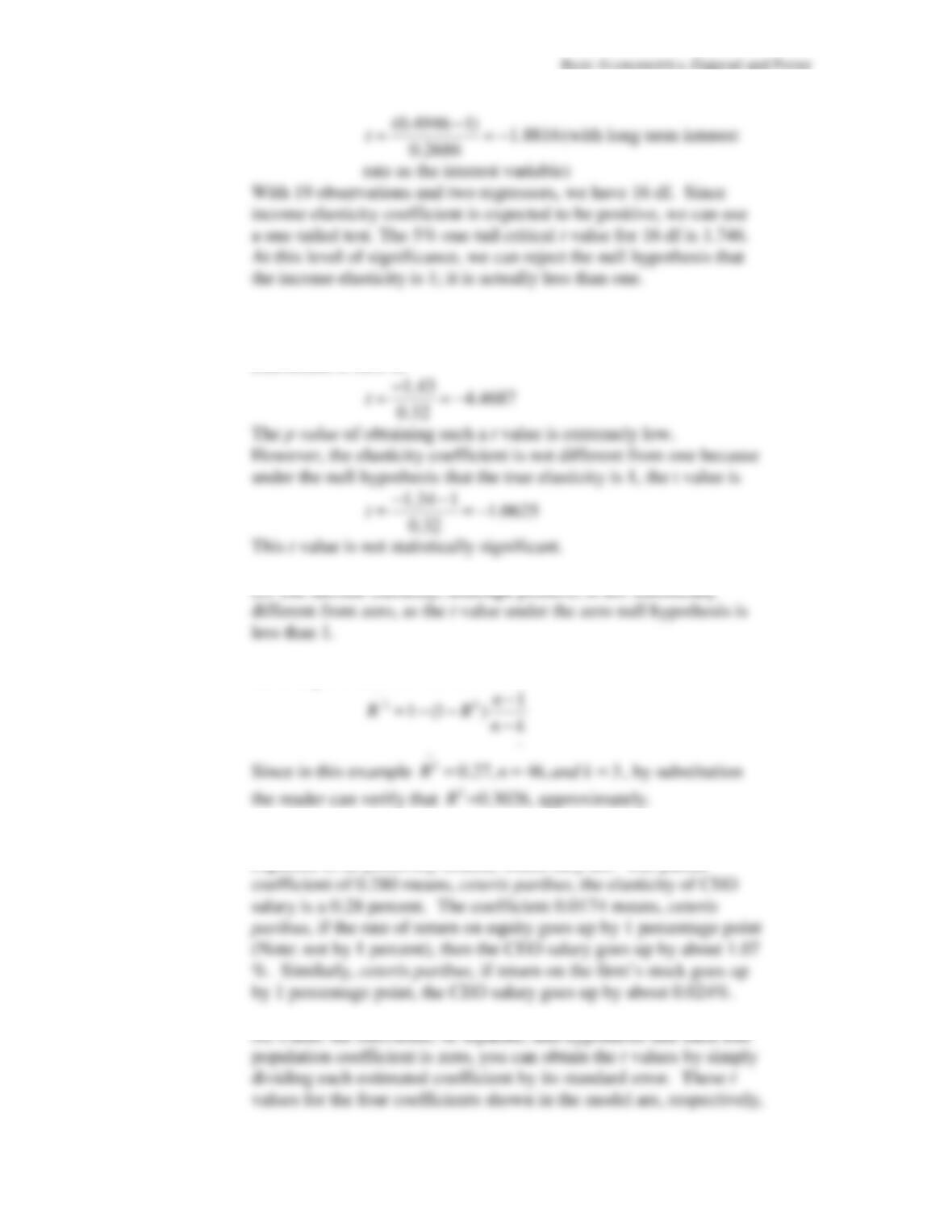
Here the null hypothesis is that the income elasticity coefficient
is unity. To test the null hypothesis we use the t test as follows:
75
8.13
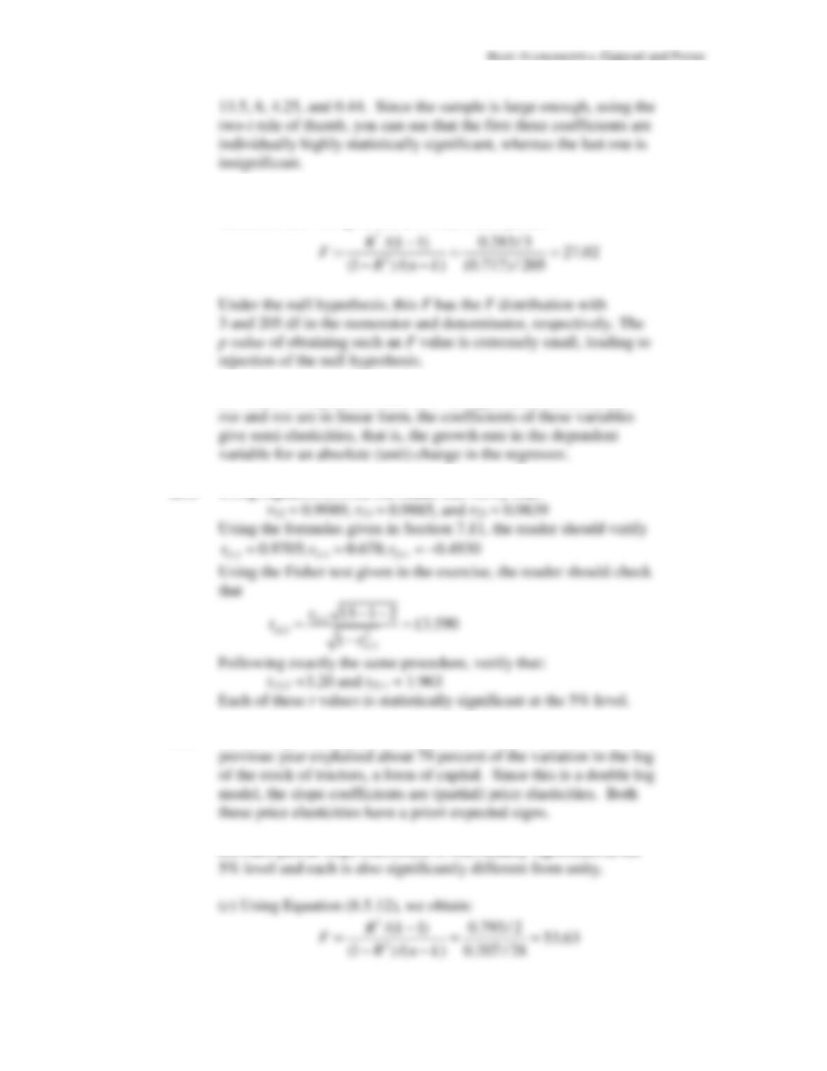
(a) The elasticity is –1.34. It is significantly different from zero, for
the t value under the null hypothesis that the true elasticity
coefficient is zero is:
(c) Using formula (7.8.4), we obtain:
8.14
(a)A priori, salary and each of the explanatory variables are
expected to be positively related, which they are. The partial
76
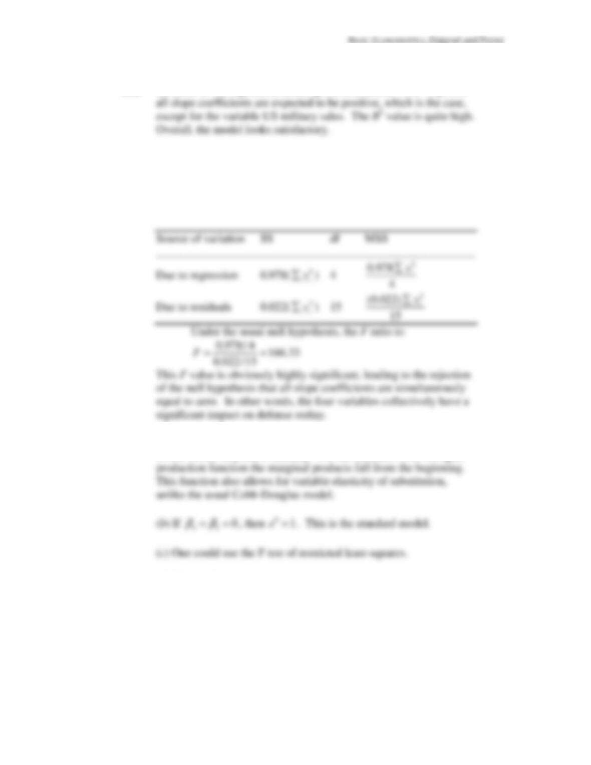
(c) To test the overall significance, that is, all the slopes are equal to
zero, use the F test given in (8.5.11), which yields:
(d)
Since the dependent variable is in logarithmic form and the
8.15
Using Equation (3.5.8), the reader can verify that:
8.16 (a) The logs of real price index and the interest rate in the
(b) Each partial slope coefficient is individually significant at the
Basic Econometrics, Gujarati and Porter
77
8.17 (a) Ceteris paribus, a 1 (British) pound increase in the prices of final
output in the current year lead on average to a 0.34 pound (or 34
(b) If you divide the estimated coefficients by their standard errors,
(c) As we will study in the chapter on distributed lag models, this
(e) Use the following (standard) elasticity formula:
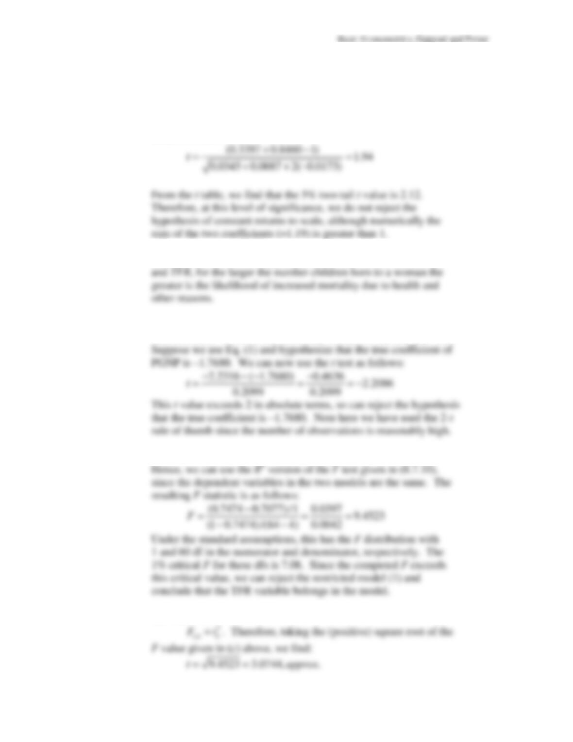
8.18 (a) Ceteris paribus, a 1 percentage point increase in the job
Basic Econometrics, Gujarati and Porter
78
(b)As in the previous exercise, under the zero null hypothesis the
(d) These are designed to capture the distributed lag effect of current
(e) The X variable may be dropped from the model because it has
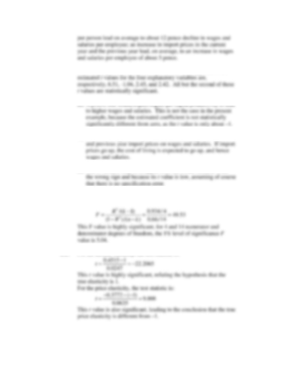
(f) Use the F test as follows:
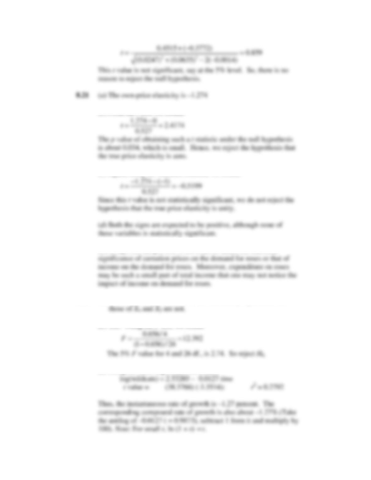
8.19 For the income elasticity, the test statistic is:
8.20 The null hypothesis is that
2 3
β β
= −
, that is,
2 3
0
β β
+ =
.
Using the t statistic given in (8.6.5), we obtain:
Basic Econometrics, Gujarati and Porter
79
(b) From the t test, we obtain:
(c) Again, using the standard formula, we obtain:
(e)Perhaps our sample size is too small to detect the statistical
8.22
(a) The coefficients of X
2
and X
3
are statistically significant, but
(b) Yes. Using the F test, we obtain
(c) Using the semi-log model, we obtain:
80
8.23
(a) Refer to the regression results given in Exercise 7.18. A priori,
(b) We can use the R
2
version of the ANOVA table given in Table
8.5 of the text.
8.24
(a) This function allows the marginal products of labor and capital
to rise before they fall eventually. For the standard Cobb-Douglas
(d)
The results are as follows:
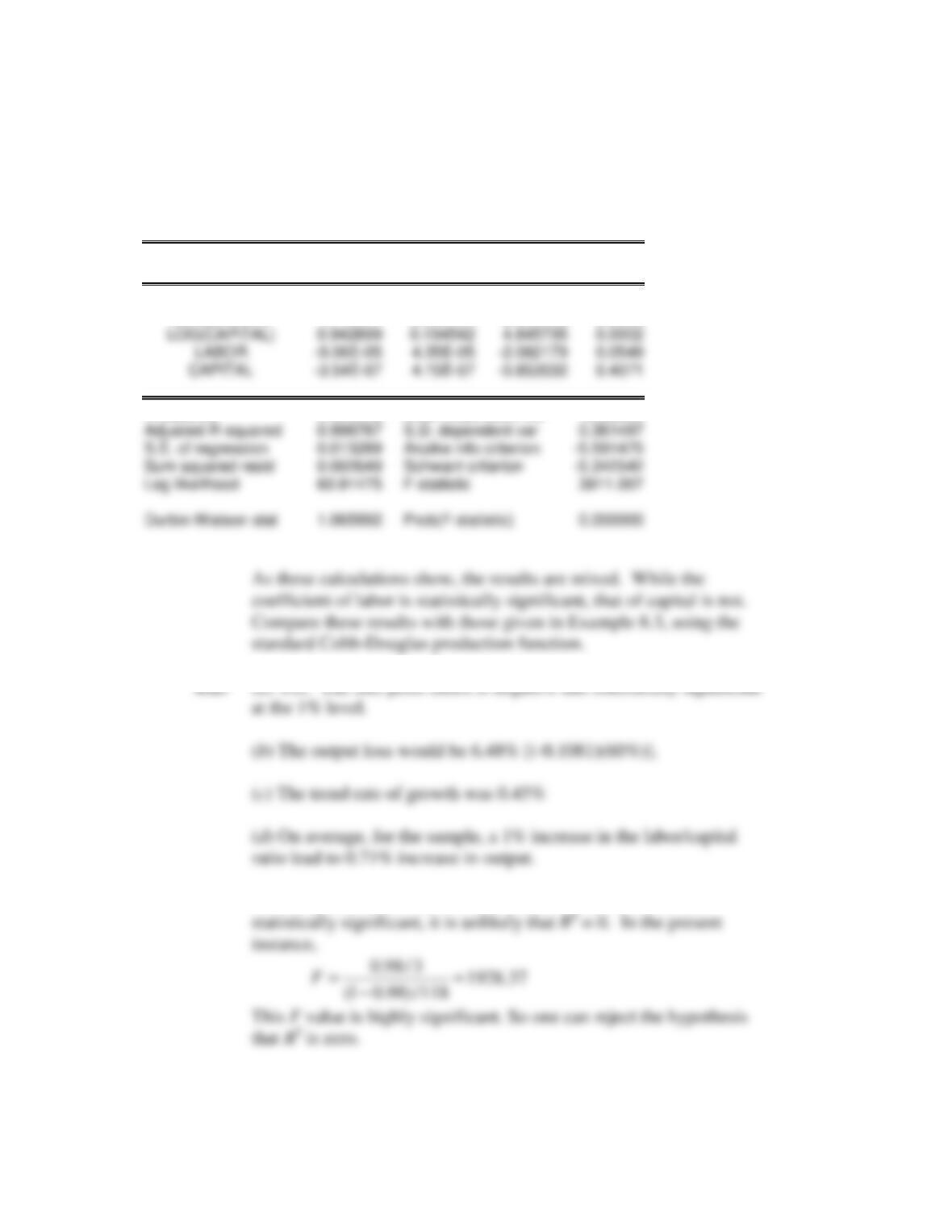
Basic Econometrics, Gujarati and Porter
81
Dependent Variable: LOG(GDP)
Sample: 1955 1974
Included observations: 20
Variable Coefficient
Std. Error
t-Statistic
Prob.
C -11.70601
2.876300
-4.069814
0.0010
LOG(LABOR) 1.410377
0.590731
2.387512
0.0306
R-squared 0.999042
Mean dependent var 12.22605
(e) See Question 8.11 above. If each individual coefficient is
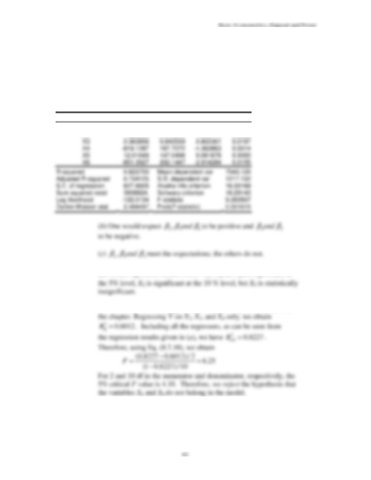
8.26
(a) The EViews3 output is as follows:
Dependent Variable: Y
Sample: 1968 1983
Included observations: 16
Variable Coefficient
Std. Error
t-Statistic
Prob.
C 5962.656
2507.724
2.377716
0.0388
X2 4.883663
2.512542
1.943714
0.0806
(d) As the regression results show,
,
X X and X
are significant at
(e) We use the methodology of restricted least-squares discussed in
8.27
(a) Since both models are log-linear, the estimated slope coefficients
represent the (partial) elasticity of the dependent variable with
respect to the regressor under consideration. For instance, the
Basic Econometrics, Gujarati and Porter
83
8.29
We will discuss only the results based on the treasury bill rate; the
results based on the long-term rate are parallel.
Note that we have put only one restriction, namely, that the
coefficient of Y in the first model is unity.
84
8.30
To use the t test given in (8.7.4), we need to know the covariance
between the two slope estimators. From the given data, it can be
shown that cov (
2 3
,
β β
∧ ∧
) = -0.3319. Applying (8.7.4) to the Mexican
data, we obtain:
8.31
(a) A priori, one would expect a positive relationship between CM
(b) The coefficients of PGNP are not very different, but that of FLR
look different. To see if the difference is real, we can use the t test.
(c)We can treat model (1) as the restricted version of model (2).
(d) Recall that
Basic Econometrics, Gujarati and Porter
85
8.32
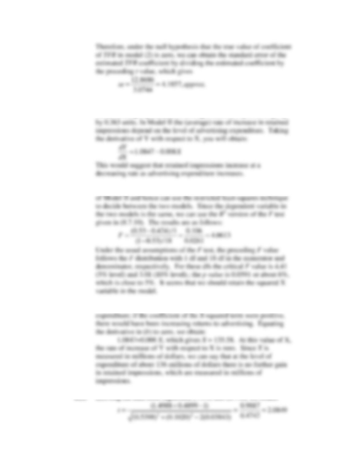
(a) In Model I the slope coefficient tells us that per unit increase in
the advertising expenditure, on average, retained impressions go up
(b) &(c)We can treat Mode I 1 as the abridged, or restricted, version
(d) As noted in (b), there are diminishing returns to advertising
Basic Econometrics, Gujarati and Porter
86
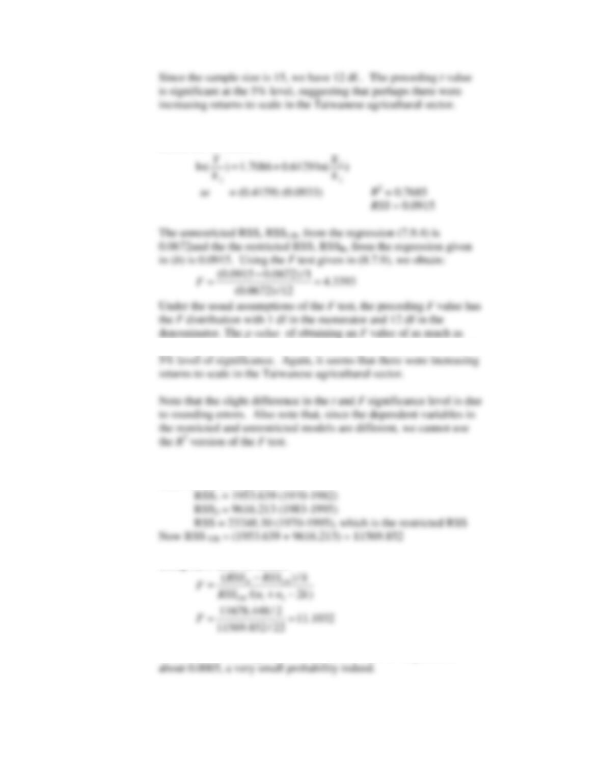
(b) Imposing the constant-returns-to-scale restriction, the regression
results are as follows:
4.34 or greater is about 0.0593 or about 6 percent, which close to the
8.34
Following exactly the steps given in Sec. 8.8, here are the various
sums of residual squares:
Using the F test, we obtain:
The p value obtaining an F value of as much as 11 or greater is
Basic Econometrics, Gujarati and Porter
87
8.35
(a) The results of the linear model are reproduced below:
(b) Use the standard elasticity formula. For example, to calculate the
income elasticity, we need to calculate:
(c) To test if the income and wealth coefficients are statistically the same,
we would compute the t statistic as follows:
Basic Econometrics, Gujarati and Porter
88
Dependent Variable: LOGC
Method: Least Squares
Sample: 1947 2000
Included observations: 54
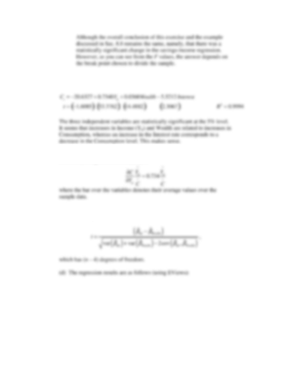
LOGC=C(1)+C(2)*LOGYD+C(3)*LOGWEALTH+C(4)*INTEREST
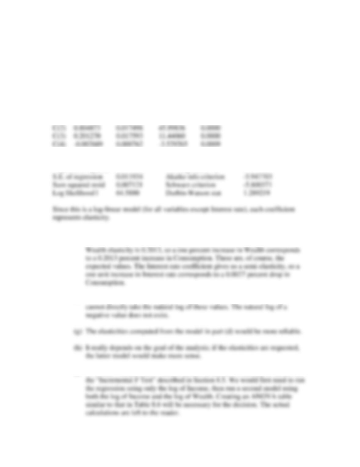
Coefficient Std. Error t-Statistic Prob.
C(1) -0.467711 0.042778 -10.93343 0.0000
R-squared 0.999560 Mean dependent var 7.826093
Adjusted R-squared 0.999533 S.D. dependent var 0.552368
(e) The Income elasticity is 0.8049, meaning that a one percent increase in
Income corresponds to a 0.8049 percent increase in Consumption. The
(f) Since there were several negative values in the Interest rate column, we
(i) To decide whether a new variable should be added to a model, we should use
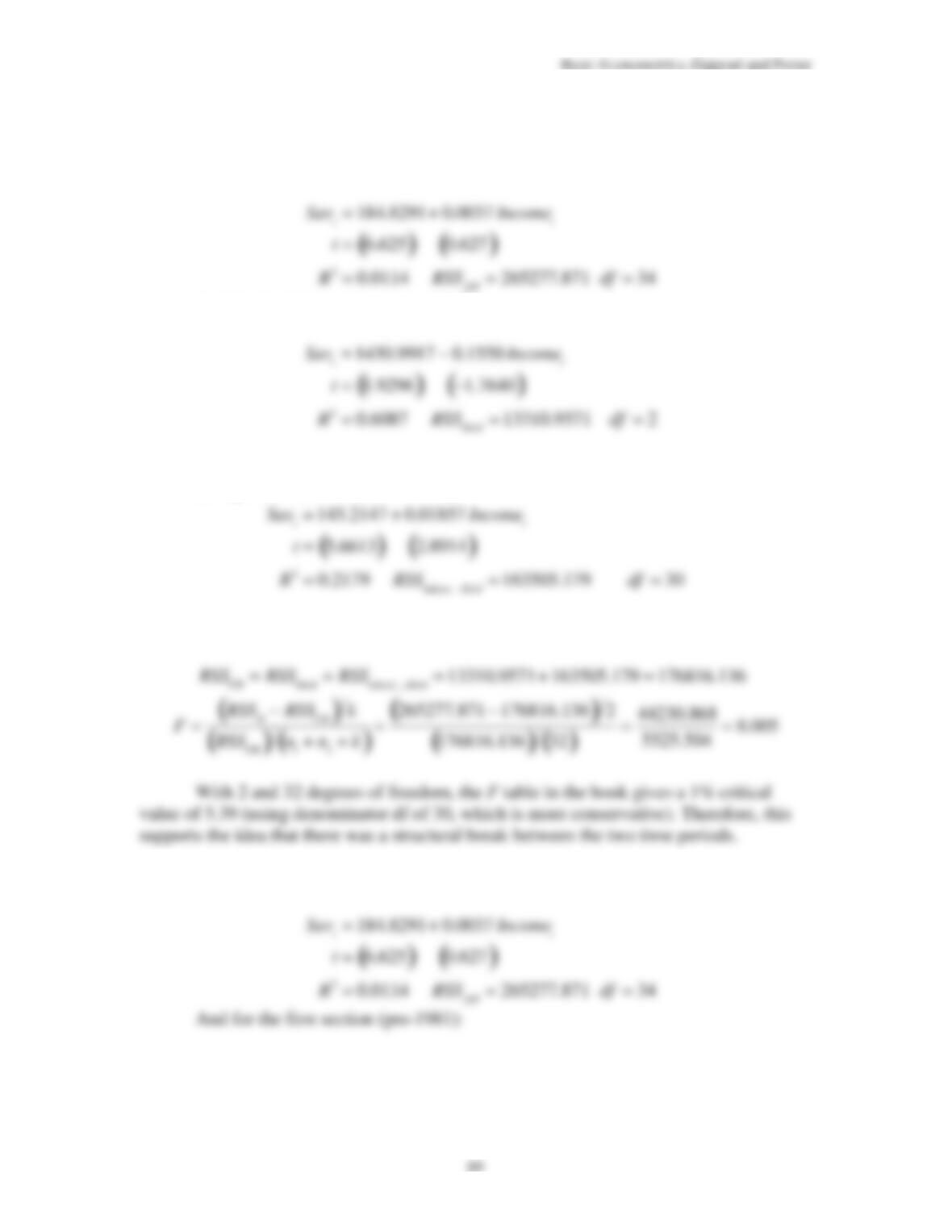
8.36 (a) The results of the full dataset model are as follows:
And for the third section (post-2002):
The last necessary piece is the regression for all the years except for the third
section (i.e., pre-2002):
The Chow test for this question is constructed as follows:
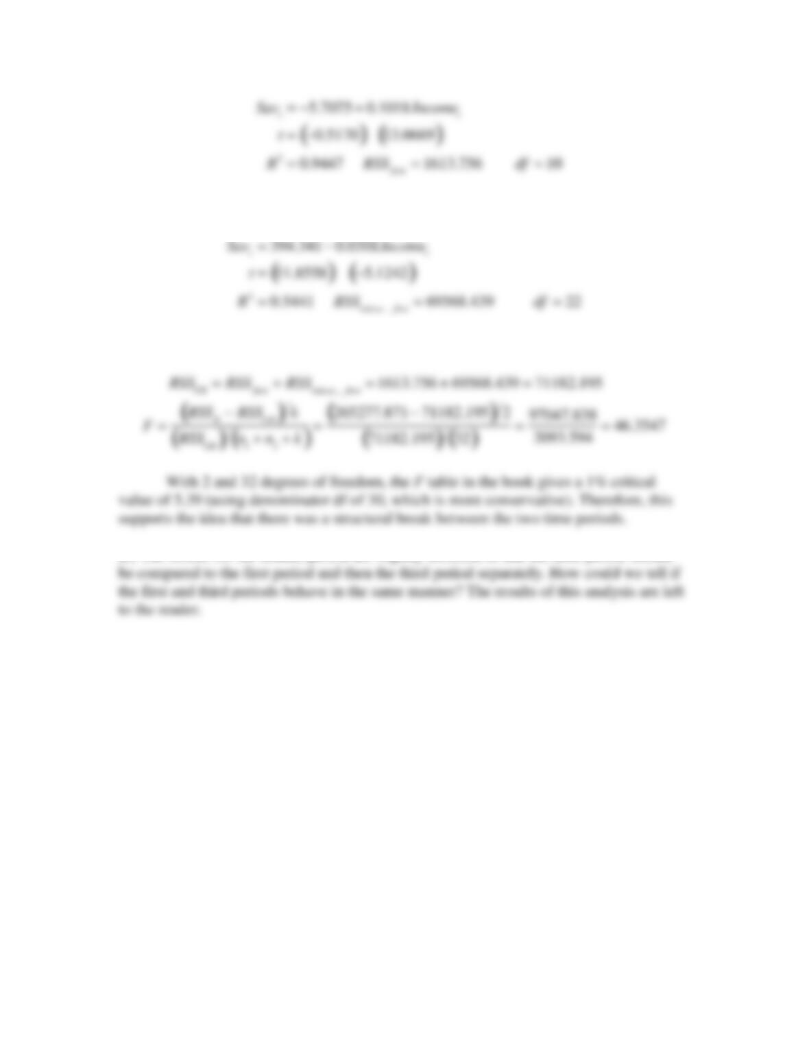
(b) The results of the full dataset model are as follows:
Basic Econometrics, Gujarati and Porter
90
The last necessary piece is the regression for all the years except for the first
section (i.e., post-1981):
The Chow test for this question is constructed as follows:
(c) The results for the middle period are slightly different in that the time period should